Welcome to Deep Bottleneck’s documentation!

Background

An introduction to artificial neural networks

Making some sorts of artificial lives, capable of acting humanly-rational, has been a long lasting dream of mankind. We started with mechanical bodies, working solely based on laws of physics, which were mostly fun creatures rather than intelligent ones. The big leap took place as we stepped in the programmable computers era; when the focus shifted to those features of human skills which were a bit more brainy. So the results became more serious and successful. Codes started beating us in some aspects of intelligence which involve memory and speed, especially when they were tested using well, and formally, structured s. But their Achilles Heel was the tasks that need a bit of intuition and our banal common sense. So, while codes were instructed to outperform us at solving elegant logical problems at which our brains are miserably weak, they failed to carry out some simple trivial tasks that we are able to do, even without consciously thinking about them. It was like we made an intangible creature who is actually intelligent, but in a different direction perpendicular to the direction of our intelligence. Thus, we thought if we really want something that act similar to us, we need to structure it just like ourselves. And that was the very reason for all the efforts that finally led to the realization of artificial neural networks (ANNs).

Unlike the conventional codes, which are instructed what to do, in a step-by-step way and by a human supervisor, neural networks learn stuff by observing data. It is almost the same as the way our brain learns doing intuitive tasks that we have no clear idea of exactly how and exactly when we have learned doing them; for example, a trivial task like recognizing a fire hydrant in a picture of a random street. And that was the way we chose to tackle the common sense problem of AI. So, what are these neural networks?

Perceptron

Let’s start with the perceptron, which is a mathematical model of a single neuron and the plainest version of an artificial neural network: a network with one single-node layer. However, from a practical point of view, a perceptron is only a humble classifier that divide input data into two categories: the ones that cause our artificial neuron fires, and the ones that does not. The procedure is like this: the perceptron takes one or multiple real numbers as input, sums over a weighted version of them, adds a constant value, bias, to the result, and then uses it as the net input to its activation function. That is the function that calculates if the perceptron is going to be activated with the inputs or not. The perceptron uses Heaviside step function as its activation function. So the output of this function is the the perceptron output.

Fig. 1. Perceptron

In language of math, a perceptron is a simple equation:

Eq. 1

where x_i is the ith input, w_i is the weight correspond to the ith input, b stands for the bias, and H is the Heaviside step function which will be activated with positive input:

Eq. 2 [1]

For the sake of neatness of the equation, we add a facial input, x₀ , which is always equal to 1 and its weight, w₀ , represent the bias value. Then we can rewrite the perceptron equation as:

Eq. 3

and simplify the diagram, by removing the addition node, assuming everyone knows that the activation function will work on the summation of inputs:

Fig. 2. Perceptron

Hands On (1)

If we have [.5, 3, -7] as inputs, and [4, .2, 9] as our weights, and the bias sets to 2, the net
input to the Heaviside step function is:

4(.5)+.2(3)+9(-7)+2 = -58.4

And since the result is negative, the perceptron output is 0.

Snippet (1)

Perceptron could be easily coded. It is just a bunch of basic math operations and an if-else
statement. Here is an example code, using Python:

import numpy as np

def perceptron(input_vector):
    '''
    This perceptron function takes a 3-element
    array in form of a row vector as its argument,
    and returns the output of the above described
    perceptron.
    '''

    # setting the parameters
    bias = 2
    weights = np.array([4, .2, 9])

    # calculating the net input to the HSFunction
    input = np.inner(input_vector, weights) + bias

    # implementing Heaviside step function
    if input < 0:
        output = 0
    else:
        output = 1

    return output


input_vector = np.array([.5, 3, -7])
print('The perceptron output is ', perceptron(input_vector))

As we did with the code, dealing with a perceptron, the input is the only variable we have. But the weights and the bias are the parameters of our perceptron and parts of its architecture. It does not necessarily mean that the weights and the bias take constant values. On the contrary, we will see that the most important, and the beauty, of perceptron is its ability to learn and this learning happens through the change of the weights and the bias.

But for now, let’s just talk about what does each of the perceptron parameters do? We can use a simple example. Assume you want to use a perceptron deciding if a specific person likes watching a specific movie or not.[2] You could define an almost arbitrary set of criteria as your perceptron input, like the movie genre, how good are the actors, and say the movie production budget. We can quantize these three criteria assuming the person loves watching comedies, so if the movie genre is comedy (1) or not (0). And the total number of prestigious awards won by the four leading/supporting actors, and the budget in million USD. The output 0 means the person, probably, does not like the movie and 1 means she, probably, does.

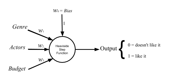
Fig. 3. A perceptron for binary classification of movies for a single Netflix user

Now it is easier to have an intuitive understanding of what each of perceptron parameters does. Weights help to give a more important factor, a heavier effect on the final decision. So for example, if the person is a huge fan of glorious fantasy movies with heavy CGI, we have to set w₁ a little bit higher. Or if she is open to discovering new talents over watching the same arrogant acting styles, we could lower down w₂ a bit. The bias role, however, is not as obvious as the weights. The simplest explanation is that bias shift the firing threshold of the perceptron or to be accurate the activation function. Suppose the intended person cares equally for the three elements of input and won’t watch a movie that fails to meet each one them. Then we have to set the bias so high that a high score in none of these three indices cannot make the perceptron fire, singly. Or if she probably would like Hobbit-kinds of movie, even though they do not fit in comedy genre, we can lower down the bias to the extent that having high scores, the Actors and the Budget could fire the perceptron together. You might think that we could do all these kind of arrangements solely using the weights. So let’s deal with this case in which all the input parameters are equal to zero. Without adding a bias term the output would be zero regardless of what we are taking in, and what we are willing to classify.

Hands On (2)

Assume we have two binary inputs, A and B, which could be either 0 or 1. What we want is to
design a perceptron that takes A and B and behaves like a NOR gate; that is the perceptron
output will be 1 if and only if both A and B are 0, otherwise the output will be 0.

It is not always guaranteed for all problems, but in this case, we could do the design in too
many different ways, with a wide variety of values as weights and the bias. One possible valid
combination of the parameters is: wA = -2, wB = -1, and the bias = 1. We can check the results:

Another valid set of parameters would be: wA = -0.5, wB = -0.5, and .4 for the bias. You can
think of many more sets of valid parameters yourself.

Now try designing this perceptron without adding bias.

The last thing to talk about is the activation function. The function is like the perceptron brain. Even though it does not do complicated calculations, but without it the perceptron is nothing but a linear combination of the inputs.[3] The activation function helps perceptron to learn. Once the perceptron parameters are set, it is able to differentiate between different sets of inputs and to make decisions via its elementary mechanism of ‘fire’ or ‘do not fire’.

That would be also fun to compare a perceptron with a neuron; provided that you do not take this comparison too seriously.[4] You can think of the inputs, naïvely, as chemoelectrical signals transmitting through dendrites (weights), reaching the neuron (Heaviside step function), if the pulse passes the threshold (bias), the neuron fires down the axon (the output is 1), otherwise it does not (the output is 0).

The Network

So… not a big deal? We have a basic classifier which it is limited to linearly separable data. Suppose we want to divide a set of samples that are, somehow, represented using a coordinate system. The perceptron would be able to do the task, if and only if, the two sets could be separated by drawing a single straight line between them.[5]

Problem (1)

Design a perceptron that takes two binary inputs, A and B and returns the XOR value of them:

So at this point, perceptron might seem a little boring. But we can make it wildly exciting with taking one step further in imitating our brain structure by connecting artificial neurons together to form a network in which each perceptron output is fed as input to another perceptron; something like this:

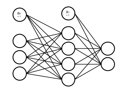
Fig. 4. An artificial neural network

As you see in the picture, the artificial neurons, or simply the nodes, are organized in layers. Nodes in a layer are not connected to each other. They are just connected to other nodes in their previous and/or next layers, except for the bias nodes. The bias nodes are not connected to their previous layer nodes, because being connected backward means their value is going to be set with the incoming flow. But bias nodes, as we see in perceptron, are conventionally set to feed 1,[6] so they are disconnected from their previous layers.

The first layer of the network is the input layer, and the last one is the output layer. Every layer in between is called a hidden layer. Note that, in the above picture, the input layer is more of a decorative setting, or a placeholder only to represent the input flow. The nodes in this layer are not actual perceptrons. They, just like the bias nodes, merely stand for input variables, and unlike the other nodes in the network, do not represent any activation function.[7] When we are counting a network layers, we only consider the layers with adjustable weights led to them. So in this case, we do not count the input layer and say it is a 2-layer neural network, or the depth of this network is 2. The number of neurons in each layer is called its width. But, just like the poor input layer, we do not include bias nodes while counting the width. So in our network the hidden layer width is 4 and the output layer width is 2.

As the depth of the network increases, it could easier deal with the more complicated patterns. The same happens when the width of layers grows. What this complex structure does is to break down the input data into small fragments and find a way to combine the most informative parts as output.

Imagine we want to estimate people income, based on their age, education, and say blood pressure. Assume we want to use the multiple linear regression method to accomplish the task. So what we do is to find how much and in which way each of our explanatory variables (i.e. age, education, and blood pressure) affects the income. That is, we reduce income to summation of our variables multiplied by their corresponding coefficient plus a bias term. Sounds good, does not work all the time. What we neglect here is the implicit relations between the explanatory variables, themselves. Like the general fact that, as people age, their blood pressure increases. Now what a neural network with its hidden layers does is to taking these relations into account. How? With chopping each input variable into pieces, thanks to many nodes in a one single layer, and letting these pieces each of which belongs to a different variable, combine together with a specific proportion, set by the weights, in the next layer. In other word, a neural network let the input variable have interaction with each other. And that is how the increase of width and the depth enable the network to handle and to construct more complex data structures.

Problem (2)

We discussed a privilege of neural networks over the multiple linear regression in doing a specific
task. Regarding the same task, would the neural network performance still have any privilege over a
multivariate nonlinear regression, which can handle nonlinear dependency of a variable on multiple
explanatory variables?

Snippet (2)

Assume we have the following network, in which all the nodes in the hidden and output layers have
Heaviside step function as their activation function:

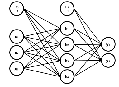
The hidden layer weights are given with the following connectivity matrix:

So according to this matrix, w32 or the weight between the second input x2 and the third node in the
hidden layer, h3, is 5. That is, x2 will be multiplied by -5, before being fed to h3. You might feel
a little uncomfortable with w32 convention of labeling and like w23 much better. But you will see
noting the destination layer index before the origin layer makes life much easier. In addition, you
can always remember that the weights are set only to adjust the value which is going to be fed to
the next layer.

And, in the same way, the following connectivity matrix gives us the output layer weights:

And the bias vectors are:

Now we want to write a code to model this network, get a numpy array with the shape of (3,) as the
input and returns the network output:

import numpy as np

# Modeling Heaviside Step function
def heaviside(z):
    '''
    This function models the Heaviside Step Function;
    it takes z, a real number, and returns 0 if it is
    a negative number, else returns 1.
    '''
    if z < 0:
        return 0
    else:
        return 1

# And vectorizing it, suitable for applying element-wise
heaviside_vec = np.vectorize(heaviside)

def ann(input_0):
    '''
    This Artificial Neural Network function takes a 3-element
    array in the form of a row vector as its argument, and returns
    a two-element row vector as its output.
    '''

    # setting the parameters
    bias_0 = np.array([2, -3, 1, .6])
    bias_1 = np.array([4, 5])
    weights_10 = np.array([[4, 3, 2], [-2, 1, .5], [2, -5, 1.2], [3, -1, 6]])
    weights_21 = np.array([[2, -1, 5, 3.2], [-4.5, 1, 3, 2]])

    # calculating the net input to the first (hidden) layer
    input_1 = np.matmul(weights_10, input_0.transpose()) + bias_0.transpose()

    # calculating the output of the first (hidden) layer
    output_1 = heaviside_vec(input_1)

    # calculating the net input to the second (output) layer
    input_2 = np.matmul(weights_21, output_1.transpose()) + bias_1.transpose()

    # calculating the output of to the second (output) layer
    output_2 = heaviside_vec(input_2)

    return output_2

So, now that we know the magic of more nodes in each layer and more hidden layers, what does stop us from voraciously extending our network? First of all we have to know that it is theoretically proven that a neural network with only one hidden layer can model any arbitrary function as accurate as you want, provided that you add enough nodes to that hidden layer.[8] However, adding more hidden layers makes life easier, both for you and your network. Then again, what is the main reason for sticking to the smallest network that would handle our problem?

With the perceptron, for example when we wanted to model a logic gate, it was a simple and almost intuitive task to find proper weights and bias. But as we mentioned before that the most important, and the beauty of a perceptron is its capacity to learn functions, without us setting the right weights and biases. It can even go further, and map inputs to desired outputs with finding and observing patterns in data that are hidden to our defective human intuition. And that is where the magical power of neural networks come from. Artificial neurons go through a trial and error process to find the most effective values as their weights and biases, regarding what they are fed and what they are supposed to return. This process takes time and would also be computationally expensive.[9] Therefore, the bigger the network, the slower and more expensive its performance. And that is the reason for being thrifty in implementing more nodes and layers in our network.

Activation Functions

Speaking of learning, how does perceptron learn? Assume that we have a dataset including samples with attributes a, b, and c. And we want to be able to train the perceptron to predict attribute c provided a and b. What the perceptron does it to start with random weights and bias. It takes the samples attributes a and b as its input and calculates the output, which is supposed to be the attribute c. Then it compares its result with the actual c, measures the error and based on the difference, it adjusts its parameters a little bit. The procedure will be repeated until the error shrinks to a desired neglectable level.

Cool! Everything seems quiet perfect, except the fact that the output of perceptron activation function is either 1 or 0. So if the perceptron parameters change a bit, its output does not change slowly, but jumps to the other possible value. Thus, the error is either at its maximum or minimum level. For making an artificial neuron trainable, we started using other functions as activation functions; functions which are, somehow, smoothed approximations of the original step function.

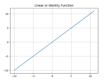
Linear or Identity Function

Earlier we talked about the absurdity of a perceptron (not to mention a network) not using an activation function, because its output would simply be a linear combination of the inputs. But, actually, there is a thing as linear or identity activation function. Imagine a network in which all nodes work with linear functions. In this case, according to linearity math, no matter how big or how elaborately-structured that network is, you can simply compress it to one single layer. However, a linear activation function could still be used in a network, if we use it as activation function of a few nodes; especially the ones in the output layer. There are cases, when we are interested in regression problems rather than classification ones, in which we want our network to have an unbounded and continuous range of outputs. Let’s return to example where we wanted to design a perceptron capable of predicting if a user wants to watch a movie or not. That was a classification problem because our desired range of output was discrete; a simple bit of 0 or 1 was enough for our purpose. But assume the same perceptron with the same inputs is supposed to predict the box office revenue. That would be a regression problem because our desired range of output is a continuous one. In such a case a linear activation function in the output layer would send out whatever it takes in, without confining it within a narrow and discrete range.

Eq. 4

Snippet (3)

Modeling the linear or identity activation function and plotting its graph:

import numpy as np
import matplotlib.pyplot as plt

def linear(z):
    '''
    This function models the Linear or Identity
    activation function.
    '''
    y = [component for component in z]
    return y


# Plotting the graph of the function for an input range
# from -10 to 10 with step size .01

z = np.arange(-10, 11, .01)
y = linear(z)

plt.title('Linear or Identity Function')
plt.grid()
plt.plot(z, y)
plt.show()

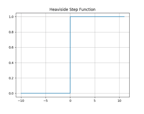
Heaviside Step Function

We already met the Heaviside step function:

Eq. 5

Snippet (4)

Modeling the Heaviside step activation function and plotting its graph:

import numpy as np
import matplotlib.pyplot as plt

def heaviside(z):
    '''
    This function models the Heaviside step
    activation function.
    '''
    y = [0 if component < 0 else 1 for component in z]
    return y


# Setting up the domain (horizontal axis) from -10 to 10
# with step size .01

z = np.arange(-10, 11, .01)
y = heaviside(z)

plt.title('Heaviside Step Function')
plt.grid()
plt.plot(z, y)
plt.show()

Sigmoid or Logistic Function

Sigmoid or logistic function is currently one of the most used activation functions, capable of being used in both hidden and output layers. It is a continuous and smoothly-changing function, and that makes it a popular option because these features let the neurons to tune its parameters at the finest level.

Eq. 6

Snippet (5)

Modeling the Sigmoid or Logistic activation function and plotting its graph:

import numpy as np
import matplotlib.pyplot as plt

def sigmoid(z):
    '''
    This function models the Sigmoid or Logistic
    activation function.
    '''
    y = [1 / (1 + np.exp(-component)) for component in z]
    return y


# Plotting the graph of the function for an input range
# from -10 to 10 with step size .01

z = np.arange(-10, 11, .01)
y = sigmoid(z)

plt.title('Sigmoid or Logistic Function')
plt.grid()
plt.plot(z, y)
plt.show()

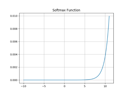
Softmax Function

Let’s go back to the movie preferences example. In the original problem setting, what we wanted to do was to know if the user likes watching a specific movie or not. So our desired output was a binary classification. Now consider a situation when we also want to check the user interest in movie using multiple level; for example: she does not like to watch the movie, she likes to watch the movie, she likes the movie so much that she would purchase the first video game produced based on the movie. And instead of a decisive answer of 0 or 1, we want a probability value for each of these three outcomes, in a way that they sum up to 1.

In this case, we cannot use a sigmoid activation function in the output layer anymore; even though the sigmoid neurons output works well as probability value, but it only handle binary classifications. Then that is exactly when we use a Softmax activation function instead; that is, when we want to do a classification task with multiple possible classes. You can think of Softmax as a cap over your network multiple, and raw, outputs, which takes them all and translates the results to a probabilistic language.

Since Softmax is designed for such a specific task, using it in hidden layers is irrelevant. In addition, as you will see in the equation, what Softmax does is to take multiple values and deliver a correlated version of them. The output values of a Softmax node are dependent on each other. That is not what we want to do with our raw stream of information in our neural network. We do not want to constrain the information flow in the network, in any possible way, when we do not have any logical reason for that. However, recently, some researchers have found a good bunch of these logical reasons to use Softmax in hidden layers.[10] But the general rule is do not use it in hidden layer as long as you do not have a clear idea of why you are doing this.[11] Anyway, this is the Softmax activation function:

Eq. 7

To have a better understanding of what is going on over there, the following diagram could be useful:

Fig. 5. Softmax layer

Snippet (6)

Modeling the Softmax activation function and plotting its graph:

import numpy as np
import matplotlib.pyplot as plt

def softmax(z):
    '''
    This function models the Softmax activation function.
    '''
    y = [np.exp(component) / sum(np.exp(z)) for component in z]
    return y


# Plotting the graph of the function for an input range
# from -10 to 10 with step size .01

z = np.arange(-10, 11, .01)
y = softmax(z)

plt.title('Softmax Function')
plt.grid()
plt.plot(z, y)
plt.show()

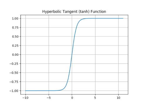
Hyperbolic Tangent or TanH Function

Hyperbolic tangent activation function or simply tanh is pretty much like the sigmoid function, with the same popularity, and the same s-like graph. In fact, as you can check with the equation, you can define the tanh function using a horizontally and vertically, scaled and shifted version of the sigmoid function. And for that reason you can model a network with tanh hidden nodes using a network with sigmoid hidden nodes and vice versa. However, unlike the sigmoid function which its output is between 0 and 1, and therefore a lovely choice for probabilistics problems, tanh output ranges between -1 and 1, and therefore is zero centered, thanks to the vertical shift we mentioned. That enables tanh function to handle negative values with its negative range. For the very same reason, training process is easier and faster with tanh nodes.

Eq. 8

Snippet (7)

Modeling the tanh activation function and plotting its graph:

import numpy as np
import matplotlib.pyplot as plt

def tanh(z):
  '''
  This function models the Hyperbolic Tangent
  activation function.
  '''
  y = [np.tanh(component) for component in z]
  return y

# Plotting the graph of the function for an input range
# from -10 to 10 with step size .01

z = np.arange(-10, 11, .01)
y = tanh(z)

plt.title('Hyperbolic Tangent (tanh) Function')
plt.grid()
plt.plot(z, y)
plt.show()

Rectified Linear Unit or ReLU Function

Rectified Linear Unit or ReLU function, currently, is the hottest activation function in the hidden layers. Mathematically, ReLU is the step function and linear function joining together at the point zero. It rectifies the linear function by shutting it down in negative range.

Eq. 9

This combination makes it benefit from the good features of both functions. That is, while ReLU enjoys the unboundness of linear function, thanks to its behavior in the negative range, it is still a nonlinear function, not a barely, hardly useful linear function. We discussed that no matter how deep and how complex is a network of linear nodes, you can compress it to a single layer network of the same linear nodes. On the other hand, a network formed of ReLU neurons, could model any function you think of. The reason is that the nonlinearity of ReLU function will be chopped into random pieces and combined in complex patterns going through hidden layers and neurons; just the same as what happens to information flow in a neural network. And that makes the network nonlinear with a desirable level of complexity. In addition, ReLU benefits its linear part the way that the linear function itself can barely make use of. As we mentioned training a network needs a steady and slow rates of change in the network output. A feature that is missing in sigmoid and tanh neurons when we move towards big negatives and positives value. At those ranges, sigmoid and tanh have asymptotic behavior which means their change rates get undesirably slow and diminish. But ReLU has a steady rate of change, albeit for the positive range. There is one more beautiful thing about ReLU behavior in negative range. Networks with sigmoid and tanh neurons are firing all the time; but a ReLU neuron just like its wet counterpart sometimes does not fire, even in the presence of a stimuli. So using ReLU we can have sparse activation networks. This property, alongside with the steady rate of change, and its simple form, enables ReLU not only to have a faster training session, but also to be computationally less expensive. Though this negative blindness of ReLU has its own issues, as well. First and most obvious, it cannot handle negative values. Secondly, we have this problem called dying ReLu, that happens in the negative range, when the rate of change becomes zero. So when a neuron produce a big enough negative output, changing its weights and bias does not show any regress or progress; just like a dead body sending out flatline.

Snippet (8)

Modeling the ReLU activation function and plotting its graph:

import numpy as np
import matplotlib.pyplot as plt

def relu(z):
    '''
    This function models the Rectified Linear Unit
    activation function.
    '''
    y = [max(0, component) for component in z]
    return y

# Plotting the graph of the function for an input range
# from -10 to 10 with step size .01

z = np.arange(-10, 11, .01)
y = relu(z)

plt.title('Rectified Linear Unit (ReLU) Function')
plt.grid()
plt.plot(z, y)
plt.show()

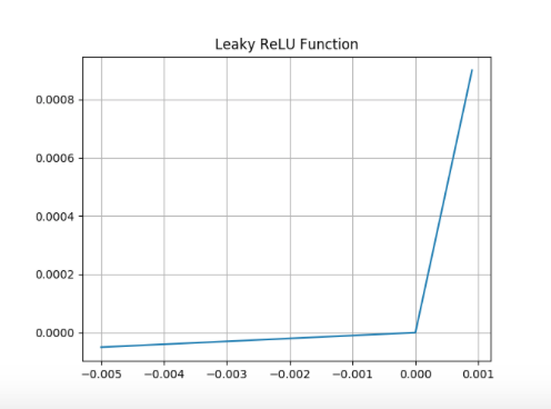
Leaky ReLU Function

And the Leaky ReLU function is here to solve the negative issues about the negative blindness of ReLU function aka dying ReLU. So instead of a flatline with zero change rate, leaky ReLU leaks a little in negative range, with an arbitrary, but gentle slope, usually set to .01. But it costs us the ‘sparse activation’ advantage of ReLU.

Eq. 10

Snippet (9)

Modeling the Leaky ReLU activation function and plotting its graph:

import numpy as np
import matplotlib.pyplot as plt

def lRelu(z):
  '''
  This function models the Leaky ReLU
  activation function.
  '''
  y = [max(.01 * component, component) for component in z]
  return y

# Plotting the graph of the function for an input range
# from -.005 to .001 with step size .001

z = np.arange(-.005, .001, .001)
y = lRelu(z)

plt.title('Leaky ReLU Function')
plt.grid()
plt.plot(z, y)
plt.show()

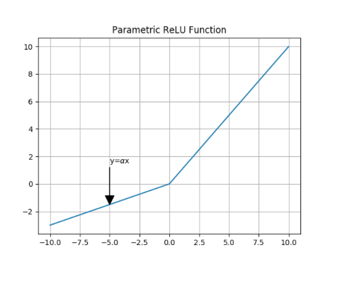
Parametric ReLU or PReLU Function

Parametric ReLU or PReLU function is a variant of the Leaky ReLU, in that the slope is not constant but it is defined as a another parameter of the network, 𝛼, which will be tuned during training just like other parameters, weights and biases.

Eq. 11

Snippet (10)

Modeling the PReLU activation function and plotting its graph:

import numpy as np
import matplotlib.pyplot as plt

def pRelu(z):
  '''
  This function models the Parametric ReLU or PReLU
  activation function with alpha equals to .3.
  '''
  y = [max(.3 * component, component) for component in z]
  return y

# Plotting the graph of the function for an input range
# from -10 to 10 with step size .01

z = np.arange(-10, 10, .01)
y = pRelu(z)

plt.title('Parametric ReLU Function')
plt.annotate(r'y=$\alpha$x', xy=(-5, -1.5), xytext=(-5, 1.5),
            arrowprops=dict(facecolor='black', width=.2))
plt.grid()
plt.plot(z, y)
plt.show()

Maxout Function

You see how PReLU was generalizing Leaky ReLU, and Leaky ReLU was, somehow, generalization of ReLU. Now, the Maxout activation function is a big step further in generalization of ReLU family of activation functions. Think about PReLU one more time, and this time try to see it as a combination of two linear functions.

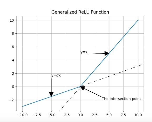
Fig. 6.

So, what ReLU family do, basically, is to take the x and compute the corresponding y, using two lines’ equations, and then pass the biggest y as the output. Now, what Maxout does, is to do the same except two things. First, Maxout won’t limit itself to only two lines. And second, those lines that Maxout work with, do not have pre-defined equations, but their characteristics like slope and y-insects will be learned. From this aspect, you can say Maxout is not just training the network, but on a lower level, it is also training the activation function, itself.

Fig. 7.

Maxout has a two-stage mechanism. There are linear nodes, at the first stage, which take the previous layer outputs (or the networks input, for sure) as their inputs, and the next stage is just a simple function, picking the maximum out.

Eq. 12

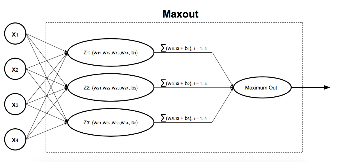
Fig. 8. Maxout inside workings

In the above picture, we have a Maxout neurons with 3 linear nodes. As you might noticed, Maxout linear nodes will be fed with net outputs of the previous layer (or network inputs), instead of being processed by weights and biases. The reason is obvious; Maxout weights and biases are shifted to its linear nodes. A network with two Maxout neurons can approximate any continuous function with an arbitrary level of accuracy.

Snippet (11)

Modeling the Maxout activation function:

import numpy as np
import matplotlib.pyplot as plt

def maxout(x, w, b):
  '''
  This function models the Maxout activation function.
  It takes input, x, the Maxout linear nodes weights, w,
  and its biases, b, all with numpy array format.
  x.shape = (1,i)
  w.shape = (n,i)
  b.shape = (1,n)
  i = the number of Maxout inputs
  n = the number of Maxout's linear nodes
  '''
  y = np.max(w @ np.transpose(x) + np.transpose(b))
  return y

Exponential Linear Unit or ELU Function

Softplus Function

Radial Basis Function

Swish Function

Arctangent Function

Hard Tangent Function

Problem (3)

Think of a new activation function with some advantages over the popular ones. Run an expriment to
compare its perfocrmance with the others. If it outperforms the hot ones, publish a paper on it.

Training

But…

Statistical Dependence

If a random variable, called X, could give any information about another random variable, say Y, we consider them dependent. The dependency of two random variables means knowing the state of one will affect the probability of the possible states of the other one. In the same way, the dependency of a random variable could be passed and also defined for a probability distribution. Investigating a possible dependency between two random variables is a difficult task. A more specific and more difficult task is to determine the level of that dependency. There are two main categories of techniques for measuring statistical dependency between two random variables. The first category mainly deals with the linear dependency and includes basic techniques like the Pearson Correlation and the Spearman’s Measure. But these techniques do not have a good performance measuring nonlinear dependencies which are more frequent in data. The second category, however, include general techniques that cover nonlinear dependencies, as well.

1. Distance Correlation

Distance correlation (dCor) is a nonlinear dependence measure and it can handle random variables with arbitrary dimensions. Not surprisingly, dCor works with the distance; the Euclidean distance. Assume we have two random variables X and Y. The first step is to form their corresponding transformed matrices, TMx and TMy. Then we calculate the distance covariance:

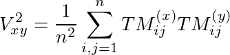
And finally, we calculate the squared dCor value as follows:

The dCor value is a real number between 0 and 1 (inclusively), and 0 means that the two variables are independent.

2. Mutual Information

Mutual information (MI) is a general measure of dependance based on the core concept of information theory, ‘entropy.’ Entropy is a measure of uncertainty, and is formulated based on the average ‘information content’ of a set of possible outcomes of an event, which is in turn, a measure of information.

Information content of the outcome x with probability P(x):

Entropy of an event with N outcomes with probabilities P1…Pn:

Mutual information is a symmetric relation between two variables and it indicates the amount of information that one random variable reveals about the other. Or in other words the reduction of uncertainty about a variable, resulted from our knowledge about another one:

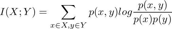
Mutual information is a symmetric and non negative value. And a zero MI means two independent variables.

Calculating MI for discrete valued variables is somewhat easy, the problem arises when we try to calculate MI, or in fact the entropy itself, for variables with real, continuous values. For working under this condition, we use the other version of MI formula which is a specific form of the more general form of Kullback-Leibler divergence and works on Probability Density Function (PDF) of joint probabilities:

However, the need for knowing PDF is another problem. In practice, we usually have access to a finite set of data spamles, and not the PDF they are representing. So before being able to calculate MI, or in essence entropy, we need to approximate the PDF itself. In this sense, the problem of estimating MI reduces to the problem of estimating PDF. In fact, most of MI estimators start with PDF estimation procedure. There are two main groups of MI estimators: parametric and non-parametric estimators. Parametric estimators are the ones that assume the probability density could be modelled with one of the most frequent distributions like Gaussian. Non-parametric estimators assume nothing about the hidden PDF.

The main approaches for estimating MI, in a non-parametric way, are methods based on histogram, adaptive partitioning, kernel density, B-spline, and k-nearest neighbor.

2.1. Histogram-based Estimation

Using a histogram is a simple, neat, and popular approach for MI estimation, which is computationally easy and efficient: we discretize the distribution into N number of bins, count the number of occurrences of samples per bin. The number of bins is an arbitrary option, best decided on, cosidering the nature of our data. Using bins with constant width make our estimation too sensitivie to the that arbitrary number of N which could lead ignoring some meaningful patterns in our data, only because some samples were interpreted within two neighboring, instead of one single bin. That is, constant bins number or their width is not sensitive to the changes in data stream, and therfore, not as efficient as the histogram estimation could potentially be. So another way is to focus on the bins width rather than their number and try to define them variably. This approach will reduce the estimation error, but would increase the complexity of the computation by adding a new problem of how to decide about the changing bin-width and how to implement the decision.

An example of using histogram estimation. Haeri, M. A., & Ebadzadeh, M. M. (2014). Estimation of mutual information by the fuzzy histogram. Fuzzy Optimization and Decision Making, 13(3), 287-318.

2.2. Adaptive Partitioning

Adaptive partitioning, as it is clear from its name, is another way of dividing data space into subsets and subsequent counting of the covered occurrences. The new thing about adaptive partitioning is that it does not confine itself to classic histogram bins, rather it feels free to use different-sized rectangular tiles to cover the data space in a way that increase the conditional independence between partitions. Partitioning is done through an iterative procedure in which after each step, the conditional independence of each tile regarding the other partitions will be examined using Chi-square statistical test.

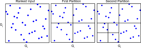
An example of adaptive partitioning procedure. He, J., Zhou, Z., Reed, M., & Califano, A. (2017). Accelerated parallel algorithm for gene network reverse engineering. BMC systems biology, 11(4), 83.

2.3. Kernel Density Estimation (KDE)

Kernel density estimation, outperforms both histogram and adaptive partitioning methods, in accuracy. But, not surprisingly, it is computationally a heavier and slower method. The main difference and advantage of KDE is its tolerance in partitioning. KDE not only does not restrict itself to rectangular, so to say, bins or any specific point in data space as the origin, and it also does not use strict lines at borders. What it uses is a kernel with an arbitrary width. This arbitrariness, again, is a weakness and makes the resulted PDF sensitive to the decision on the kernel width. In the next step, KDE calculates one of different possible probability densities including Gaussian, Rectangular, and Epanechnikov around each data samples, add them up together to obtain a smooth PDF over all data samples from the superposition of these kernels. The resulted PDF is of high quality because of a smaller MSE rate.

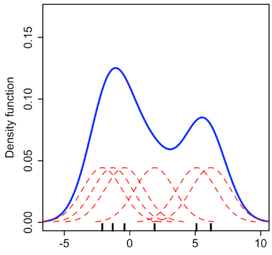
Implementing KDE. http://daveakshat.blogspot.com/2013/04/convolution-probabilty-density.html

2.4. B-Spline

This method is simply using basis spline function to approximate the underlying PDF. A B-spline function separates dataspce with equally-distanced hypotetical lines (or thier counterparts in case of working with higer dimensional data) and try to regress the data points trapped in each interval with a polynomial function. These continuous functions form the PDF which we will use later for calculating MI. B-spline results usually improve by increasing the function order. But when the final goal is estimating MI, increasing the order to more than 3 won’t affect the result.

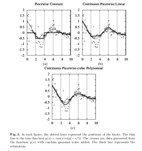
An example of using splines with different orders to approximate an underlying function. Venelli, A. (2010, April). Efficient entropy estimation for mutual information analysis using B-splines. In IFIP International Workshop on Information Security Theory and Practices (pp. 17-30). Springer, Berlin, Heidelberg.

2.5. K-Nearest Neighbor (KNN)

K-Nearest Neighbor method has a big difference with the previous MI estimators. It bypasses the PDF approximation phase and jumps right into the MI calculation phase. There is a family of KNN-based method for estimating MI, but the most popular one is the KSG. KSG uses a slightly modified MI formula in which the marginal and joint entropies for each data sample for each of two random variables are calculated using KL entropy estimator. KL entropy estimator computes entropy based on KNN idea, and with regards to the K smallest distances in a data set. KSG results are of high precision and it is a great option while working with high dimensional data. KSG is capable of working with irregular PDFs and it, currently, is one of the most popular MI estimators.

The pseudocode for KSG. Gao, W., Kannan, S., Oh, S., & Viswanath, P. (2017). Estimating mutual information for discrete-continuous mixtures. In Advances in Neural Information Processing Systems (pp. 5986-5997).

How does ‘Statistical Dependance’ help understanding deep learning?

Artificial neural networks were originaly designed to somehow replicate our biological neural network. Researcher were also partially hopeful to be able, by this replication, to learn a thing or two about the inner workings of human brain. But the irony is that the ANNs, especially the ‘deep neural network’ generation, turned to such a successful computational structure that its excellent behavior became a mysterious puzzle itself.

Publishing three papers in 1999, 2015, and 2017, Tishby offered and explored an idea for demystifying the DNN excellency using information theory concepts. According to Tishby, the key feature of a DNN is its capacity to forget. It is crucial to forget because not all the input information is necessary for accomplishing the task at the output layer. For example, consider a classification task in which pictures of cats and dogs are fed into the network and the network should decide whether an input image represent a cat or a dog. Feeding a cat photo into the network, we enter not only information about the shape of the animal but also its color. However, we know that whatever color is the animal, it does not affect its catish nature. For good results, the network should recognize and focus on the, probably the animal ear shape or face structure. So there is lots of information available which not only consume computational efforts, but also might mislead a network in its final decision. So what is important here, is not the ‘information,’ rather the ‘relevant’ information. That is where the ‘forgetting’ thing seems essential.

To make his point, Tishby offers his readers a Markov-chain perspective of a DNN and then tries to assess how the information flow is traveling through the DNN layers. For proving his theory of forgetting irrelevant data, he needed to show that the information flow in each layer leaves behind some parts of the input content and becomes more similar to the information content of the desired labels. Tishby calls this procedure ‘successive refinement of relevant information’. For doing so, he made use of mutual information concept. The mutual information between each layer and the input/labels was calculated using a histogram estimator with constant and equally-spaced bin size.

Tishby, then, defined a new plot for representing the information flow in a deep network, called ‘information plane.’ The x-axis of the information plane corresponds to I(X;T) which is mutual information between the input and the hidden layers. The y-axis corresponds to I(T;Y) which is mutual information between the hidden layers and the labels. In simple words, the horizontal axis tells us how much information a specific hidden layer is conveying about the input data and the vertical axis tells us how much information a specific hidden layer is conveying about the labels.

What Tishby seems to find out through his information plane was dazzling:

https://www.quantamagazine.org/new-theory-cracks-open-the-black-box-of-deep-learning-20170921/ | |

The information plane shows a really interesting path of information flow or in fact mutual information ratio, especially, in the last hidden layers of DNN. It seems like the last layers start with a very low mutual information with the input data which is understandable, because the input data passing through all the layers with all their neurons had enough time to scattered enough not to be statistically similar/dependance to the original data at the input layer. So, these layers start with low I(X;T) but spend training time to gather enough information and generalize the ‘concepts’ in the input data. Tishby called this phase of increasing I(X;T) ‘fitting phase.’

Then, as you see, the last hidden layers start to lose input information, but at the same time gain information, or in fact structures of information, similar to the labels data. So their I(T;Y) keep increasing while I(X;T) is decreasing. Tishby calls this phase, ‘compression phase,’ in which the network lose irrelevant data and compress its information flow. And according to Tishby, this phase change and ‘forgetting’ process is what makes the deep learning so efficient and successful.

---

[1]	We usually denote an activation function input with the letter z, rather than good old x, in order to prevent any confusion of the function input with the perceptron/network inputs.

[2]	For motivation, assume Netflix offered a US$1,000,000 prize for designing this perceptron.

[3]	Plus bias which in no-activation-function case, is itself an irrelevant factor.

[4]

Yes, the original idea was to imitate the way our brain works, but let’s be honest with ourselves, do we know how our brain works? But that aside, perceptron and ANNs have adopted a couple of important and effective macro features of our brain structure, like not being a simple/linear transmitter but getting activated with specific functions/patterns or the network structure itself which is made up of, generally, uniform elements.

[5]	Or a plane/hyperplane for 3 and more dimensions.

[6]	The value 1 is arbitrary, and only more convenient to work with. But whatever other value you assign to the bias nodes it should be constant during the flow of data through the network.

[7]	However, we will see that this is not a rule.

[8]	And provided that the nodes’ activation functions are nonlinear.

[9]	Both in an abstract and also a physical sense.

[10]	Xu, K., Ba, J., Kiros, R., Cho, K., Courville, A., Salakhudinov, R., … & Bengio, Y. (2015, June). Show, attend and tell: Neural image caption generation with visual attention. In International conference on machine learning (pp. 2048-2057).

[11]	Compare with the fact that you can use, say, a sigmoid neuron, almost wherever in a network that you want, without being sure of what you are doing!

Literature summary

1. On the information bottleneck theory of deep learning (Saxe 2018)

[Saxe2018]

1.1 Key points of the paper

• none of the following claims of Tishby ([Tishby2015]) holds in the general case:

  1. deep networks undergo two distinct phases consisting of an initial fitting phase and a subsequent compression phase
  2. the compression phase is causally related to the excellent generalization performance of deep networks
  3. the compression phase occurs due to the diffusion-like behavior of stochastic gradient descent

• the observed compression is different based on the activation function: double-sided saturating nonlinearities like tanh yield a compression phase, but linear activation functions and single-sided saturating nonlinearities like ReLU do not.

• there is no evident causal connection between compression and generalization.

• the compression phase, when it exists, does not arise from stochasticity in training.

• when an input domain consists of a subset of task-relevant and task-irrelevant information, the task-irrelevant information compress although the overall information about the input may monotonically increase with training time. This compression happens concurrently with the fitting process rather than during a subsequent compression period.

1.2 Most important experiments

1. Tishby’s experiment reconstructed:

   • 7 fully connected hidden layers of width 12-10-7-5-4-3-2
   • trained with stochastic gradient descent to produce a binary classification from a 12-dimensional input
   • 256 randomly selected samples per batch
   • mutual information is calculated by binning the output activations into 30 equal intervals between -1 and 1
   • trained on Tishby’s dataset
   • tanh-activation function

2. Tishby’s experiment reconstructed with ReLU activation:

   • 7 fully connected hidden layers of width 12-10-7-5-4-3-2
   • trained with stochastic gradient descent to produce a binary classification from a 12-dimensional input
   • 256 randomly selected samples per batch
   • mutual information is calculated by binning the output activations into 30 equal intervals between -1 and 1
   • ReLu-activation function

3. Tanh-activation function on MNIST:

   • 6 fully connected hidden layers of width 784 - 1024 - 20 - 20 - 20 - 10
   • trained with stochastic gradient descent to produce a binary classification from a 12-dimensional input
   • non-parametric kernel density mutual information estimator
   • trained on MNIST dataset
   • tanh-activation function

4. ReLU-activation function on MNIST:

   • 6 fully connected hidden layers of width 784 - 1024 - 20 - 20 - 20 - 10
   • trained with stochastic gradient descent to produce a binary classification from a 12-dimensional input
   • non-parametric kernel density mutual information estimator
   • trained on MNIST dataset
   • ReLU-activation function

1.3 Presentation

Click here to open presentation as PDF document.

2. Estimating mutual information

[Kraskov2004]

2.1 Introduction

• Kraskov suggests an alternative mutual information estimator that is not based on binning but on k-nearest neighbour distances.

• Mutual information is often used as a measure of independence between random variables. We note that mutual information is zero if and only if two random variables are strictly independent.

• Mutual information has some well known properties and advantages since it has close ties to Shannon entropy (see appendix of the paper), still estimating mutual information is not always that easy.

• Most mutual information estimation techniques are based on binning, which often leads to a systematic error.

• Consider a set of \(N\) bivariate measurements, \(z_i = (x_i, y_i), i = 1,...,N\), which are assumed to be iid (independent identically distributed) realizations of a random variable \(Z=(X,Y)\) with density \(\mu (x,y)\). \(x\) and \(y\) can be scalars or elements of a higher dimensional space.

• For simplicity we say that \(0 \cdot \log(0) = 0\) in order to consider probability density functions that do not have to be strictly positive.

• The marginal densities of \(X\) and \(Y\) can be denoted as follows:

  \[\mu_x(x) = \int \mu (x,y) dy \ \text{and } \ \mu_y(y) = \int \mu (x,y) dx.\]

• Therefore we can define mutual information as

  \[I(x,y) = \int_Y \int_X \mu (x,y) \cdot \log \dfrac{\mu (x,y)}{\mu_x (x) \mu_y(y)} dx dy.\]

• Note that the base of the logarithm sets the unit in which information is measured. That means that if we want to measure in bits, we have to take base 2. In the following we will take the natural logarithm for estimating mutual information.

• Our aim is to estimate mutual information without any knowledge of the probability functions \(\mu\), \(\mu_x\) and \(\mu_y\). The only information we have is set \(\{ z_i \}\).

2.2 Binning

• Binning is an often used technique to estimate mutual information. Therefore we partition the supports of \(X\) and \(Y\) into bins of finite size by considering the finite sum:

  \[I(X,Y) \approx I_{\text{binned}} (X,Y) \equiv \sum_{i,j} p(i,j) \log \dfrac{p(i,j)}{p_x(i)p_y(j)},\]

  where \(p_x(i) = \int_i \mu_x (x) dx, p_y(j) = \int_j \mu_y(y)\) and \(p(i,j) = \int_i \int_j \mu (x,y) dx dy\) (meaning \(\int_i\) is the integral over bin \(i\)).

• Set \(n_x(i)\) to be the number of points falling into bin i of \(X\) and analogous to that set \(n_y(j)\) to be the number of points falling into bin j of \(Y\). Moreover, \(n(i,j)\) is the number of points in their intersection.

• Since we do not know the exact probability density function, we approximate them with \(p_x(i) \approx \frac{n_x(i)}{N}\), \(p_y(j) \approx \frac{n_y(j)}{N}\), and \(p(i,j) \approx \frac{n(i,j)}{N}\).

• For \(N \rightarrow \infty\) and bin sizes tending to zero, the binning approximation (\(I_{\text{binned}}\)) indeed converges to \(I(X,Y)\). Constraint: all densities exist as proper functions.

• Note that the bin size do not have to be the same for each bin. Adaptive bin sizes actually lead to much better estimations.

2.3 Kraskov estimator

• The Kraskov estimator uses k-nearest neighbour statistics to estimate mutual information.

• The basic idea is to estimate \(H(X)\) from the average distance to the k-nearest neighbour, averaged over all \(x_i\).

• Since mutual information between two random variables can also be written as

  \[I(X,Y) = H(X) + H(Y) - H(X,Y),\]

  with \(H(X)= - \int \mu (x) \log \mu (x) dx\) being the Shannon entropy, we can estimate the mutual information by estimating the Shannon entropy for \(H(X)\), \(H(Y)\) and \(H(X,Y)\). This estimation would mean that the errors made in the individual estimates would presumably not cancel. Therefore, we proceed a bit differently:

• Assume some metrics to be given on the spaces by \(X, Y\) and \(Z=(X,Y)\).

• For each point \(z_i=(x_i,y_i)\) we rank its neighbours by distance \(d_{i,j} = ||z_i - z_j||: d_{i,j_1} \leq d_{i,j_2} \leq d_{i,j_3} \leq ...\). Similar rankings can be done in the subspaces \(X\) and \(Y\).

• Furthermore, we will use the maximum norm for the distances in the space \(Z=(X,Y)\), i.e.

  \[||z-z'||_{\max} = \max \{ ||x - x'||, ||y - y'||\},\]

  while any norms can be used for \(||x - x'||\) and \(||y - y'||\).

• We make further notations: \(\frac{\epsilon (i)}{2}\) is the distance between \(z_i\) and its \(k\)-th neighbour. \(\frac{\epsilon_x (i)}{2}\) and \(\frac{\epsilon_y (i)}{2}\) denote the distance between the same points projected into the \(X\) and :math:`Y`subspaces.

• Note that \(\epsilon(i)=\max \lbrace \frac{\epsilon_x (i)}{2}, \frac{\epsilon_y (i)}{2}\rbrace\).

• In the following, two algorithms for estimating mutual information will be taken into account:

  • In the first algorithm, the numbers of points \(x_j\) whose distance from \(x_i\) is strictly less than \(\frac{\epsilon (i)}{2}\) is counted and called \(n_x(i)\). Analogous for \(y\).

  • By \(<...>\) the averages over all \(i \in [1,...,N]\) and over all realisations of random samples is denoted:

    \[<...> = \dfrac{1}{N} \sum_{i=1}^N E[...(i)].\]

  • The mutual information can then be estimated with:

    \[I^{(1)}(X,Y) = \psi (k) - <\psi (n_x + 1) + \psi (n_y + 1)> + \psi (N).\]

  • In the second algorithm \(n_x(i)\) and \(n_y(i)\) are replaced by the number of points that satisfy the following equations:

    \[||x_i - x_j|| \leq \dfrac{\epsilon_x (i)}{2} \ \text{and} \ ||y_i - y_j|| \leq \dfrac{\epsilon_y (i)}{2}\]

  • Then mutual information can be estimated via

    \[I^{(2)}(X,Y) = \psi (k) - 1/k - <\psi (n_x) + \psi (n_y)> + \psi (N).\]

• Generally, both estimates give similar results. But it proves that \(I^{(1)}\) has the tendency to have slightly smaller statistical errors, but larger systematic errors. This means that when we are interested in very high dimensions, we better should use \(I^{(2)}\).

3. SVCCA: singular vector canonical correlation analysis

[Raghu2017]

3.1 Key points of the paper

• They developed a method that analyses each neuron’s activation vector (i.e. the scalar outputs that are emitted on input data points). This analysis gives an insight into learning dynamics and learned representation.

• SVCCA is a general method that compares two learned representations of different neural network layers and architectures. It is either possible to compare the same layer at different time steps, or simply different layers.

• The comparison of two representations fulfills two important properties:

  • It is invariant to affine transformation (which allows the comparison between different layers and networks).
  • It is fast to compute, which allows more comparisons to be calculated than with previous methods.

3.2 Experiment set-up

• Dataset: mostly CIFAR-10 (augmented with random translations)
• Architecture: One convolutional network and one residual network
• In order to produce a few figures, they decided to design a toy regression task (training a four hidden layer fully connected network with 1D input and 4D output)

3.3 How SVCCA works

• SVCCA is short for Singular Vector Canonical Correlation Analysis and therefore combines the Singular Value Decomposition with a Canonical Correlation Analysis.

• The representation of a neuron is defined as a table/function that maps the inputs on all possible outputs for a single neuron. Its representation is therefore studied as a set of responses over a finite set of inputs. Formally, that means that given a dataset \(X = {x_1,...,x_m}\) and a neuron \(i\) on layer \(l\), we define \(z^{l}_{i}\) to be the vector of outputs on \(X\), i.e.

  \[z^{l}_{i} = (z^{l}_{i}(x_1),··· ,z^{l}_{i}(x_m)).\]

  Note that \(z^{l}_{i}\) is a single neuron’s response over the entire dataset and not an entire layer’s response for a single input. In this sense the neuron can be thought of as a single vector in a high-dimensional space. A layer is therefore a subspace of \(\mathbb{R}^m\) spanned by its neurons’ vectors.

1. Input: takes two (not necessarily different) sets of neurons (typically layers of a network)

   \[l_1 = {z^{l_1}_{1}, ..., z^{l_{m_1}}_{l_1}} \text{ and } l_2 = {z^{l_2}_{1}, ..., z^{l_{m_2}}_{l_2}}\]

2. Step 1: Use SVD of each subspace to get sub-subspaces \(l_1' \in l_1\) and \(l_2' \in l_2\), which contain of the most important directions of the original subspaces \(l_1, l_2\).

3. Step 2: Compute Canonical Correlation similarity of \(l_1', l_2'\): linearly transform \(l_1', l_2'\) to be as aligned as possible and compute correlation coefficients.

4. Output: pairs of aligned directions \((\widetilde{z}_{i}^{l_1}, \widetilde{z}_{i}^{l_2})\) and how well their correlate \(\rho_i\). The SVCCA similarity is defined as

   \[\bar{\rho} = \frac{1}{\min(m_1,m_2)} \sum_i \rho_i .\]

3.4 Results

• The dimensionality of a layer’s learned representation does not have to be the same number than the number of neurons in the layer.
• Because of a bottom up convergence of the deep learning dynamics, they suggest a computationally more efficient method for training the network - Freeze Training. In Freeze Training layers are sequentially frozen after a certain number of time steps.
• Computational speed up is successfully done with a Discrete Fourier Transform causing all block matrices to be block-diagonal.
• Moreover, SVCCA captures the semantics of different classes, with similar classes having similar sensitivities, and vice versa.

[SBD+18]

Andrew Michael Saxe, Yamini Bansal, Joel Dapello, Madhu Advani, Artemy Kolchinsky, Brendan Daniel Tracey, and David Daniel Cox. On the information bottleneck theory of deep learning. In International Conference on Learning Representations. 2018. URL: https://openreview.net/forum?id=ry_WPG-A-.

[KraskovStogbauerGrassberger04]

Alexander Kraskov, Harald Stögbauer, and Peter Grassberger. Estimating mutual information. \pre , 69:066138, June 2004. arXiv:cond-mat/0305641, doi:10.1103/PhysRevE.69.066138.

[RaghuGilmerYosinskiSohlDickstein17]

M. Raghu, J. Gilmer, J. Yosinski, and J. Sohl-Dickstein. SVCCA: Singular Vector Canonical Correlation Analysis for Deep Learning Dynamics and Interpretability. ArXiv e-prints, June 2017. arXiv:1706.05806.

[TishbyZaslavsky15]

N. Tishby and N. Zaslavsky. Deep Learning and the Information Bottleneck Principle. ArXiv e-prints, March 2015. arXiv:1503.02406.

Contributing

Extending the framework

There are several possibilities to extend the framework. In the following the structure of the framework is shown to allow an easy extension of the basic modules. There are five types of modules that can be included quite easy, they are listed in the table below: Each module requires a module level load method to be defined, that passes the hyperparameters from the sacred configuration to the constructor of the class.

dataset:The datasets live in the deep_bottleneck.dataset folder and require a load-method returning a training and a test dataset. model:The models live in in the deep_bottleneck.model folder and require a load-method as well. But in this case the load-method returns a trainable keras-model. estimator:The mutual information estimators live in the deep_bottleneck.mi_estimator folder and require a load-method as well. The load-method should return an estimator that is able to compute the mutual information based on a dataset and is described in more detailed by a hyperparameter called discretization_range. callback:Callbacks can be used for different kinds of tasks. They live in the deep_bottleneck.callbacks folder and are used to save the needed information during the training or to influence the training process (e.g. early stopping). They need to inherit from keras.callbacks.Callback. plotter:Plotters are using the saved data of the callbacks to create the different plots. They live in the deep_bottleneck.plotter folder and need a load method returning a plotter-class inheriting from deep_bottleneck.plotter.base.BasePlotter.

To add a new module, it needs to be added into the respective folder. Then the configuration parameter needs to be set to the import path of the module. If the path is correctly defined and the module has a matching interface, it will automatically be imported in experiment.py and conduct its tasks. More about the interfaces and the existing methods in the API-documentation.

Git workflow

This workflow describes the process of adding code to the repository.

1. Describe what you want to achieve in an issue.

2. Pull the master to get up to date.

   1. git checkout master
   2. git pull

3. Create a new local branch with git checkout -b <name-for-your-branch>. It can make sense to prefix your branch with a description like feature or fix.

4. Solve the issue, most probably in several commits.

5. In the meantime there might have been changes on the master branch. So you need to merge these changes into your branch.

   1. git checkout master
   2. git pull to get the latest changes.
   3. git checkout <name-for-your-branch>
   4. git merge master. This might lead to conflicts that you have to resolve manually.

6. Push your branch to github with git push origin <name-for-your-branch>.

7. Go to github and switch to your branch.

8. Send a pull request from the web UI on github.

9. After you received comments on your code, you can simply update your pull request by pushing to the same branch again.

10. Once your changes are accepted, merge your branch into master. This can also be done by the last reviewer that accepts the pull request.

Git commit messages

Have a look at this guideline.

Most important:

• Single line summary starting with a verb (50 characters)
• Longer summary if necessary (wrapped at 72 characters).

Editors like vim enforce these constraints automatically.

Style Guide

Follow PEP 8 styleguide. It is worth reading through the entire styleguide, but the most importand points are summarized here.

Naming

• Functions and variables use snake_case
• Classes use CamelCase
• Constants use CAPITAL_SNAKE_CASE

Spacing

Spaces around infix operators and assignment

• a + b not a+b
• a = 1 not a=1

An exception are keyword arguments

• some_function(arg1=a, arg2=b) not some_function(arg1 = a, arg2 = b)

Use one space after separating commas

• some_list = [1, 2, 3] not some_list = [1,2,3]

In general PyCharm’s auto format (Ctrl + Alt + l) should be good enough.

Type annotation

Since Python 3.5 type annotation are supported. They make sense for public interfaces, that should be kept consistent.

def add(a: int, b: int) -> int:

Docstrings

Use Google Style for docstrings in everything that has a somewhat public interface.

Clean code

And here our non exhaustive list to guidelines to write cleaner code.

1. Use meaningful variable names
2. Keep your code DRY (Don’t repeat yourself) by abstracting into functions and classes.
3. Keep everything at the same level of abstraction
4. Functions without side effects
5. Functions should have a single responsibility
6. Be consistent, stick to conventions, use a styleguide
7. Use comments only for what cannot be described in code
8. Write comments with care, correct grammar and correct punctuation
9. Write tests if you write a module

Experiment workflow

1. Define a hypothesis
2. Define set of parameters that is going to stay fixed
3. Define parameter to change (including possible values for the parameter)
4. Create a meaningful name for the experiment (group of experiment, name of parameter tested)
5. Make sure you set a seed (Pycharm: in run options append: “with seed=0”)
6. Program experiment (set parameters) using our framework
7. Commit your changes locally to obtain commit hash: this is going to be logged by sacredboard
8. Make sure your experiment is logged to the database
9. Start the experiment
10. Interpret and document results in a notebook. Include relevant plots using the artifact viewer. Make sure the notebook is completely executed.
11. Move your notebook to docs/experiments, so it will be automatically included in the documentation.
12. Push your local branch to github - to make all commits available to everyone

Documentation

To build the documentation run:

$ cd docs
$ make html

A short restructeredText reference. There is also a longer video tutorial

If you added new packages and want to add them to the API documentation use:

$ sphinx-apidoc -o docs/api_doc/ deep_bottleneck deep_bottleneck/credentials.py deep_bottleneck/experiment.py deep_bottleneck/demo.py

Make sure to change the header of modules.rst back to “API Documentation”.

User guide

Installation

Environment

To run the experiment you need to install the required dependencies. We highly recommend that you use a virtual environment as provided by conda.

To create your environment run:

$ conda create -n deep-bottleneck python=3.6
$ conda activate deep-bottleneck

Then in your environment run:

$ pip install -r requirements/dev.txt

Sacred setup

When running experiments, the hyperparameters, metrics and plots are managed through Sacred and are stored in a mongoDB database. Though you can setup your mongoDB instance however you want, it is most conveniently done through the provided Docker files. This will not only get you started with mongoDB in no time, but will also set up a mongo-express interface to conveniently manage your database and sacredboard to monitor your runs. In order to use them you need to

1. Install Docker Engine.
2. Install Docker Compose.
3. Navigate to the directory with the setup files.

$ cd infrastructure/sacred_setup/

4. If you plan to expose the mongoDB to the internet you should edit the .env file and replace all values with more secure values.

5. Run docker-compose:

   docker-compose up -d
   

This will pull the necessary containers from the internet and build them. This may take several minutes. Afterwards mongoDB should be up and running. mongo-express should now be available on port 8081, accessible by the user and password you set in the .env file (ME_CONFIG_BASICAUTH_USERNAME and ME_CONFIG_BASICAUTH_PASSWORD). Sacredboard should be available on port 5000.

The current setup is optimized for running experiments locally. When you want to log results to a remote server, you should change the port mapping in the docker-compose.yml file. Note that this will expose your database to the internet. Simply remove the localhost prefixes form all port mappings, e.g. replace:

ports:
  - 127.0.0.1:5000:5000

by

ports:
  - 5000:5000

5. You are ready to run some exciting experiments!

Importing and exporting from mongoDB

The following section is meant to help you migrate your data from one server to another. If you are just starting you can skip this section.

To export data from your mongo container run

$ docker run --rm --link <container_id>:mongo --network <network_id> -v /root/dump:/backup mongo bash -c 'mongodump --out /backup --uri mongodb://<username>:<password>@mongo:27017/?authMechanism=SCRAM-SHA-1'

make sure you you create the output folder, in this case /root/dump beforehand. You also need to look up the id of your current mongo container using docker ls and find the id of the network is running is using docker network ls. Then replace <username> and <password> by the values you originally set in your .env.

To import data again run following the same steps as above.

$ docker run --rm --link <container_id>:mongo --network <network_id> -v /root/dump:/backup mongo bash -c 'mongorestore /backup --uri mongodb://<username>:<password>@mongo:27017/?authMechanism=SCRAM-SHA-1'

How to use the framework

Running experiments

The idea of the project is based on the concepts presented by Tishby. To reproduce the basic setup of the experiments one can simply start experiment.py.

If all the required packages are installed properly and the program is started, different things should happen.

1. First the required modules of the framework are imported based on the defined configuration (more about configurations in “Adding new Experiments”).
2. A neural network is trained using the defined dataset. The progress of this process is also logged in the console.
3. During the training process the required data is saved in regular time-steps to the local filesystem.
4. Given the saved data (e.g. the activations) it is possible to compute the mutual information of the different layer and the input/output.
5. Using this different plots as e.g. the information plane plot are created and saved simultaneously in the filesystem and in the database. The results of the experiments can be looked up either in the deep_bottleneck/plots folder (only the plots of the last runs are saved) or using eval_tools as described below.

Evaluation tools

To make the rich results generated by the experiments accessible, we created an evaluation tool. It lets you query experiments based on id, name or other configuration parameters and lets you view the generated plots, metrics and videos conveniently in Jupyter notebooks. To get you started have a look at deep_bottleneck/eval_tools_demo.ipynb.

Adding new experiments (config)

Configuration

During the exploration of Tishby’s idea already a lot of experiments have been done, but there are still many things one can do using this framework. To define a new experiment a new configuration needs to be added. The existing configurations are saved in the deep_bottleneck/configs folder. To add a new configuration a new JSON file is required. The currently relevant parts of the configuration and their effects are explained in the following table.

epochs:Number of epochs the model is trained for. Most of the experiments for the harmonics dataset used 8000 epochs. batch_size:Batch size used during the training process. Most dominant batch size in our experiments was 256. architecture:Architecture of the trained model. Defined as a list of integers, where every integer defines the number of neurons in one layer. It is important to notify that an additional readout layer is automatically added (with the number of neurons corresponding to the number of classes in the dataset). The basic architecture for the harmonics dataset is [10, 7, 5, 4, 3]. optimizer:The optimizer used for the training of the neural network. Possible values are “sgd”, or “adam”. learning_rate:The learning rate of the optimizer. Default values are 0.0004 for harmonics and 0.001 for mnist. activation_fn:The activation-function used to train the model. The following activation function are implemented: tanh, relu, sigmoid, softsign, softplus, leaky_relu, hard_sigmoid, selu, relu6, elu and linear. model:The parameter which defines the basic model-choice. Currently only different architectures of feed-foreward-networks can be used. So the possible choices right now are models.feedforward and models.feedforward_batchnorm, the actual architecture is defined by the architecture parameter. dataset:The parameter which defines the dataset used for training. Currently implemented datasets are harmonics, mnist, fashion_mnist and mushroom. estimator:The estimator used for the computation of the mutual information. Because mutual information cannot be computed analytically for more complex networks, it is necessary to estimate it. Possible estimators are mi_estimator.binning, mi_estimator.lower, mi_estimator.upper. discretization_range:  The different estimators have a different hyperparameter to add artificial noise to the estimation. This parameter is used as a placeholder for the different hyperparameter. A typical value is 0.07 for binning and 0.001 for upper and lower. callbacks:A list of additional callbacks as for example early stopping. Needs to defined as a list of paths to the callbacks, as e.g. [callbacks.early_stopping_manual]. n_runs:Number of runs the experiment is repeated. The results will be averaged over all runs to compensate for outliers.

Executing multiple experiments

Using these parameters one should be able to define experiments as desired. To execute the experiment(s) one could simply start des experiment.py but mainly due to our usage of external hardware resources (Sun grid engine) we had to develop another way to execute experiments. We created two python files: run_experiment.py and run_experiment_local.py, which can run either a single experiment or a group of experiments. For the local execution of experiments with run_experiment_local.py one needs to switch to the deep_bottleneck folder by:

$ cd deep_bottleneck

and then execute experiments by either pointing to a specific JSON file defining the experiment, e.g.:

$ python run_experiments.py -d configs/basic.json

or pointing at a directory containing all the experiments one wants to execute, e.g.:

$ python run_experiments.py -d configs/mnist

In that case all the JSONs in the folder and in its sub-folders are recursively executed.

Running experiment on the Sun grid engine

In case one uses a sun grid engine to execute the experiments it is possible to start run_experiments.py on the engine in the same way with as described above. The experiments will get submitted to the engine using qsub. In that case it is important to make sure that an /output/-folder exists on the directory-level of the experiment.sge file.

Additionally it might be important to run experiments that are repeatable and will return the same results in every run. Because the basic step of the framework is to train a neural network, including some kind of randomness the results of two runs might be different even though they are based on the same configuration. To avoid misconceptions it is possible to set a seed for each experiment, simply by using:

$ python experiment.py with seed=0

(the exact seed is arbitrary, it just needs to be consistent). In case that one of the run_experiment files is used this step is done for you, but even in the other cases some IDEs allow to set script-parameters for normal executions of a specific file, such that it is not required to start the experiment.py out of the command-line.

Documentation on how to run an experiment on grid

1. Open console.

2. Connect with Server via ssh. Your username should be your Rechenzentrums Login, as well as your password should be the corresponding password.:

   $ ssh rz_login_username@gate.ikw.uos.de
   

3. If you want to run something on the grid for the first time, follow steps 4 - 7. Otherwise go directly to 8.

4. Go to the following folder:

   $ cd net/projects/scratch/summer/valid_until_31_January_2019
   

5. Create a new folder with your Rechenzentrum username.:

   $ mkdir rz_login_username
   

6. Go into your folder and clone the git repository.:

   $ cd rz_login_username
   $ git clone https://github.com/neuroinfo-os/deep-bottleneck.git
   

7. Create a folder in deep-bottleneck/deep_bottleneck that you call output.:

   $ cd deep-bottleneck/deep_bottleneck
   $ mkdir output
   

8. Go into the following folder:

   $ cd net/projects/scratch/summer/valid_until_31_January_2019/deep_bottleneck/deep_bottleneck
   

9. Make sure you created a config-file that defines your parameter settings that you want to test. These should be in the following folder:

   $ deep_bottleneck/deep_bottleneck/configs/cohort_xx (xx - set a number and document your experiment in read the docs)
   

10. Activate the dneck environment:

    $ source activate dneck
    

If that does not work than check your $PATH and see if net/projects/scratch/summer/valid_until_31_January_2019/bottleneck/miniconda/bin is already added to your path. If not:

$ export PATH=$PATH:/net/projects/scratch/summer/valid_until_31_January_2019/bottleneck/miniconda/bin

11. In order to run the experiment type:

    $ python run_experiments.py -c configs/cohort_xx
    

Choose your config file.

12. In order to see where your experiment is in the queue, check with:

    $ qstat
    

13. If experiment fails, check your output folder for console output. Delete data in output folder regularly.

Glossary

Information Theory Basics

This glossary is mainly based on MacKay’s Information Theory, Inference and Learning Algorithms. If not marked otherwise, all information below can be found there.

Prerequisites: random variable, probability distribution

A major part of information theory is persuing answers to problems like “how to measure information content”, “how to compress data” and “how to communicate perfectly over imperfect communcation channels”.

At first we will introduce some basic definitions.

The Shannon Information Content

The Shannon information content of an outcome \({x}\) is defined as

\[h(x) = \log_2 \frac{1}{P(x)}.\]

The unit of this measurement is called “bits”, which does not allude to 0s and 1s.

Ensemble

We extend the notion of a random variable to the notion of an ensemble. An ensemble \({X}\) is a triplet \((x, A_X, P_X)\), where \(x\) is just the variable denoting an outcome of the random variable, \(A_X\) is the set of all possible outcomes and \(P_X\) is the defining probability distribution.

Entropy

Let \(X\) be a random variable and \(A_X\) the set of possible outcomes. The entropy is defined as

\[H(X) = \sum_{x} p(x) \ log_2\left(\frac{1}{p(x)}\right).\]

The entropy describes how much we know about the outcome before the experiment. This means

\[\begin{split}H(X) = 0 &\iff \text{One outcome has a probability of 100%.} \\ H(X) = log_2(|A_X|) &\iff \text{All events have the same probability.}\end{split}\]

The entropy is bounded from above and below: \(0 \leq H(X) \leq log_2(|A_X|)\). Notice that entropy is defined as the average Shannon information content of an outcome and therefore is also measured in bits.

Entropy for two dependent variables

Let \(X\) and \(Y\) be two dependent random variables.

joint entropy

\[H(X,Y) = \sum_{x,y} p(x,y) \ log_2\left(\frac{1}{p(x,y)}\right)\]

conditional entropy if one variable is observed

\[H(X|y=b) = \sum_{x} p(x|y=b) \ log_2\left(\frac{1}{p(x|y=b)}\right)\]

conditional entropy in general

\[\begin{split}H(X|Y) &= \sum_{y} p(y) \ H(X|y=y) \\ &= \sum_{x,y} p(x,y) \ log_2\left(\frac{1}{p(x|y)}\right)\end{split}\]

chain rule for entropy

\[\begin{split}H(X,Y) &= H(X) + H(Y|X) \\ &= H(Y) + H(X|Y)\end{split}\]

Mutual Information

Let \(X\) and \(Y\) be two random variables. The mutual information between these variables is then defined as

\[\begin{split}I(X;Y) &= H(X) - H(X|Y) \\ &= H(Y) - H(Y|X) \\ &= H(X) + H(Y) - H(X,Y)\end{split}\]

The mutual information describes how much uncertainty about the one variable remains if we observe the other. It holds that

\[I(X;Y) = I(Y;X) I(X;Y) \geq 0\]

The following figure gives a good overview:

Mutual information overview.

Kullback-Leibler divergence

Let \(X\) be a random variable and \(p(x)\) and \(q(x)\) two probability distributions over this random variable. The Kullback-Leibler divergence is defined as

\[D_{KL}(p||q) = \sum_{x} p(x) \ log_2\left(\frac{p(x)}{q(x)}\right)\]

The Kullback-Leibler divergence is often called relative entropy and denotes “something” like a distance between two distributions:

\[\begin{split}&D_{KL}(p||q) \geq 0 \\ &D_{KL}(p||q) = 0 \iff p=q\end{split}\]

Yet it is not a real distance as symmetry is not given.

Typicality

We introduce the “Asymptotic equipartion” principle which can be seen as a law of large numbers. This principle denotes that for an ensemble of \(N\) independent and identically distributed (i.i.d.) random variables \(X^N \equiv (X_1, X_2, \dots, X_N)\), with \(N\) sufficiently large, the outcome \(x = (x_1, x_2, \dots , x_N)\) is almost certain to belong to a subset of \(\mathcal{A}_X^N\) with \(2^{NH(X)}\) members, each having a probability that is ‘close to’ \(2^{-NH(X)}\).

The typical set is defined as

\[T_{N \beta} \equiv \{ x \in \mathcal{A}_X^N : | \frac{1}{N} \log_2 \frac{1}{P(x)} - H | < \beta \}.\]

The parameter \(\beta\) sets how close the probability has to be to \(2^{-NH}\) in order to call an element part of the typical set, \(\mathcal{A}_X\) is the alphabet for an arbitrary ensemble \(X\).

Shannon’s Source Coding Theorem

Mathematical Terms in Tishby’s Experiments

Stochastic Gradient Descent

Spherical Harmonic power spectrum [Tishby (2017) 3.1 Experimental setup]

TODO

O(3) rotations of the sphere [Tishby (2017) 3.1 Experimental setup]

TODO

Experiments

Description of cohorts

The experiments are structured in different cohort, containing one specific variation of parameters. To show the aim of the cohorts and to simplify the access of the saved artifacts using the artifact-viewer the following table offers a simple description for each cohort.

Cohort	Description
cohort_1	Comparison of upper, lower and binning as different estimator. Additionally the hyperparameter of the estimators are varied. All experiments are done for relu and tanh using sgd as optimizer.
cohort_2	Comparison of training-, test- and full-dataset as base for the mi-computation. All experiments are done for relu and tanh using sgd as optimizer.
cohort_3	Comparison of upper, lower and binning as different estimator. Additionally the hyperparameter of the estimators are varied. All experiments are done for relu and tanh using adam as optimizer.
cohort_4	Comparison of training-, test- and full-dataset as base for the MI-computation. All experiments are done for relu and tanh using Adam as optimizer.
cohort_5	Comparison of different standard activation functions. All experiments are done using adam as optimizer.
cohort_6	Comparison of basic architectures. All experiments are done for relu and tanh using adam as optimizer.
cohort_7	Comparison of different hyperparameter for max-norm regularization. All experiments are done for relu and tanh using adam as optimizer.
cohort_8	Comparison of architecture with batchnorm and without batchnorm. All experiments are done for relu and tanh using adam as optimizer.
cohort_9	Comparison of architecture with batchnorm and without batchnorm. All experiments are done for relu and tanh using adam as optimizer.
cohort_10	Comparing weight norm for max_norm_weights = 0.9 and max_norm_weights = 0.6.
cohort_11
cohort_12
cohort_13	Effect of weight renormalization on activity patterns. Experiments for relu and tanh using adam as optimizer.
cohort_14

Comparison of infoplanes for different estimators

import sys
sys.path.append('../..')
from deep_bottleneck.eval_tools.experiment_loader import ExperimentLoader
from deep_bottleneck.eval_tools.utils import format_config, find_differing_config_keys
import matplotlib.pyplot as plt
from io import BytesIO

loader = ExperimentLoader()

import numpy as np
import pandas as pd

all_experiments = [[1318,1328,1327,1320,1333,1315,1325,1319,1321,1323], # binning tanh
                  [1326,1329,1316,1330,1331,1317,1332,1334,1324,1322], # binning relu
                  [1368,1369,1370,1371,1372,1375,1373,1374,1376,1377], # kde tanh
                  [1354,1358,1359,1361,1362,1363,1364,1365,1367,1366], # kde relu
                  [1454,1441,1451,1453,1455,1448,1459,1442,1458,1447], # EDGE tanh
                  [1452,1445,1446,1440,1449,1443,1444,1457,1450,1456]  # EDGE relu
                ]

label_list = ['Estimator: binning, Activation function: tanh',
             'Estimator: binning, Activation function: relu',
             'Estimator: KDE, Activation function: tanh',
             'Estimator: KDE, Activation function: relu',
             'Estimator: EDGE, Activation function: tanh',
             'Estimator: EDGE, Activation function: relu',
             ]

all_means = []
for experiment_set in all_experiments:
    experiments = loader.find_by_ids(experiment_set)
    set_df = []
    for i, experiment in enumerate(experiments):
        infoplane = experiment.artifacts['information_measures_test'].show()
        set_df.append(infoplane)

    df_concat = pd.concat(set_df)

    by_row_index = df_concat.groupby(df_concat.index)
    set_mean = by_row_index.mean()

    all_means.append(set_mean)

plt.rcParams.update({'font.size': 22})
fig, ax = plt.subplots(figsize=(24,28))

for ax_id, set_mean in enumerate(all_means):

    plt.subplot(3,2,ax_id+1)
    measures = set_mean.groupby(['epoch', 'layer']).mean()

    total_epochs = measures.index.get_level_values('epoch')[-1] + 1  # epoch index starts at 0
    sm = plt.cm.ScalarMappable(cmap='gnuplot', norm=plt.Normalize(vmin=0, vmax=total_epochs))
    sm.set_array([])

    for epoch_nr, mi_measures in measures.groupby(level=0):
        color = sm.to_rgba(epoch_nr)

        xmvals = np.array(mi_measures['MI_XM'])
        ymvals = np.array(mi_measures['MI_YM'])

        plt.plot(xmvals, ymvals, color=color, alpha=0.1, zorder=1)
        plt.scatter(xmvals, ymvals, s=20, facecolors=color, edgecolor='none', zorder=2)

        plt.title(label_list[ax_id])
        plt.xlabel('I(X;M)')
        plt.ylabel('I(Y;M)')
        plt.xlim([0, 12])
        plt.ylim([0, 1])

    fig.colorbar(sm, label='Epoch')

plt.tight_layout()
plt.show()

EDGE individiual runs

fig, ax = plt.subplots(5,2, figsize = (20,50))
ax = ax.flat
experiment_ids = [1345,1344,1346,1352,1351,1348,1347,1353,1350,1349]

experiments = loader.find_by_ids(experiment_ids)
differing_config_keys = find_differing_config_keys(experiments)

for i, experiment in enumerate(experiments):
    img = plt.imread(BytesIO(experiment.artifacts['infoplane_train'].content))
    ax[i].axis('off')
    ax[i].imshow(img)
    ax[i].set_title(format_config(experiment.config, *differing_config_keys),
                    fontsize=20)

plt.show()

fig, ax = plt.subplots(5,2, figsize = (20,50))
ax = ax.flat
experiment_ids = [1314,1339,1336,1338,1337,1335,1340,1341,1342,1343]

experiments = loader.find_by_ids(experiment_ids)
differing_config_keys = find_differing_config_keys(experiments)

for i, experiment in enumerate(experiments):
    img = plt.imread(BytesIO(experiment.artifacts['infoplane_train'].content))
    ax[i].axis('off')
    ax[i].imshow(img)
    ax[i].set_title(format_config(experiment.config, *differing_config_keys),
                    fontsize=20)


plt.show()

Cohort 10

Comparing weight norm

import sys
sys.path.append('../..')
from deep_bottleneck.eval_tools.experiment_loader import ExperimentLoader
from deep_bottleneck.eval_tools.utils import format_config, find_differing_config_keys
import matplotlib.pyplot as plt
from io import BytesIO

import pandas as pd
import numpy as np

loader = ExperimentLoader()

experiment_ids = [943,944,945,946,947,948,949]
experiments = loader.find_by_ids(experiment_ids)
differing_config_keys = find_differing_config_keys(experiments)

experiments[0].config

{'activation_fn': 'tanh',
 'architecture': [10, 7, 5, 4, 3],
 'batch_size': 256,
 'callbacks': [],
 'dataset': 'datasets.harmonics',
 'discretization_range': 0.07,
 'epochs': 8000,
 'estimator': 'mi_estimator.binning',
 'initial_bias': 0,
 'learning_rate': 0.0004,
 'max_norm_weights': 0.9,
 'model': 'models.feedforward',
 'n_runs': 5,
 'optimizer': 'adam',
 'plotters': [['plotter.informationplane', []],
  ['plotter.snr', []],
  ['plotter.informationplane_movie', []],
  ['plotter.activations', []],
  ['plotter.activations_single_neuron', []]],
 'seed': 0}

fig, ax = plt.subplots(4,2, figsize=(14, 34))
ax = ax.flat

for i, experiment in enumerate(experiments):
    img = plt.imread(BytesIO(experiment.artifacts['infoplane_train'].content))
    ax[i].axis('off')
    ax[i].imshow(img)
    ax[i].set_title(format_config(experiment.config, *differing_config_keys),
                    fontsize=16)
plt.tight_layout()
plt.show()

Effect of different initial bias settings for relu

import sys
sys.path.append('../..')
from deep_bottleneck.eval_tools.experiment_loader import ExperimentLoader
from deep_bottleneck.eval_tools.utils import format_config, find_differing_config_keys
import matplotlib.pyplot as plt
from io import BytesIO

import pandas as pd
import numpy as np

loader = ExperimentLoader()

experiment_ids = []
e_id = 1077
for i in range(44):
    experiment_ids.append(e_id+i)
experiment_ids.append(1125)
print(experiment_ids)

experiment_ids_median = [1077,1079,1080,1083,1087,1093,1120]
experiment_ids_mean = [1138,1136,,,1134,1148,]

experiment_ids = [1077,1138,1079,1136,1080,,1083,,1087,1134,1093,1148,1120,]

experiments = loader.find_by_ids(experiment_ids)

[1077, 1078, 1079, 1080, 1081, 1082, 1083, 1084, 1085, 1086, 1087, 1088, 1089, 1090, 1091, 1092, 1093, 1094, 1095, 1096, 1097, 1098, 1099, 1100, 1101, 1102, 1103, 1104, 1105, 1106, 1107, 1108, 1109, 1110, 1111, 1112, 1113, 1114, 1115, 1116, 1117, 1118, 1119, 1120, 1125]

differing_config_keys = find_differing_config_keys(experiments)

For this experiment we varied the initial bias parameter of the hidden layers with an otherwise standard setting of the parameters under a relu activation function. Varying the initial bias it interesting, as this shifts the preactivation of the layers by the specified bias output = activation(dot(input, kernel) + bias). This, in turn, affects the proportion of preactivations that end up in the saturation regime of the respective activation function. We hypothesize therefore that the inital bias can have an effect on the compression of a layer. In the case of relu, when the initial_bias=0, approximately half of the preactivations are negative and mapped to 0. This induces “immediate” compression, as it was discussed for example in notebook 9.analyze_entropy. By shifting the preactivations with the (positive) initial_bias parameter, we can supress immediate compression. Below the informationplane plots for different settings of the initial bias parameter are shown.

fig, ax = plt.subplots(7,2, figsize=(14, 34))
ax = ax.flat

for i, experiment in enumerate(experiments):
    img = plt.imread(BytesIO(experiment.artifacts['infoplane_train'].content))
    ax[i].axis('off')
    ax[i].imshow(img)
    #ax[i].set_title(format_config(experiment.config, *differing_config_keys),
    #                fontsize=16)

plt.tight_layout()
plt.show()

---------------------------------------------------------------------------
KeyError                                  Traceback (most recent call last)
<ipython-input-24-a3842bf7d890> in <module>
      3
      4 for i, experiment in enumerate(experiments):
----> 5     img = plt.imread(BytesIO(experiment.artifacts['infoplane_train'].content))
      6     ax[i].axis('off')
      7     ax[i].imshow(img)

KeyError: 'infoplane_train'

experiments[0].artifacts['infoplane_movie_train'].show()

experiments[0].artifacts

The informationplane plots shows two qualitaively different patterns. For negative initial bias settings as well as for initial bias settings wth large positive magnitude all gradients remain 0 for the entire training process, therefore not changing any weights in the network. In this setting mutual information of the resepctive layers stays constant over the entire process. Here, we only look at informationplane plots that show a some dynamic of the mutual inforamtion values over time, with inital_bias=0 as a reference. For the penultimate layer and initial_bias=0.2, 1 and 2 we can observe a decrease in mutual information with the input in the later stages of training (from epoch 1000 onwards). Does this movement towards the upper left in the information plane correspond to the network gradually learning weights and biases which push activations towards the neagtive spectrum?

fig, ax = plt.subplots(6,2, figsize=(14, 34))
ax = ax.flat

for i, experiment in enumerate(experiments):
    img = plt.imread(BytesIO(experiment.artifacts['infoplane_test'].content))
    ax[i].axis('off')
    ax[i].imshow(img)
    ax[i].set_title(format_config(experiment.config, *differing_config_keys),
                    fontsize=16)
plt.tight_layout()
plt.show()

In the following we will have a close look on the activations of experiment with initial_bias=2, experiment_id=865

bias2 = loader.find_by_id(865)
bias2.config

{'activation_fn': 'relu',
 'architecture': [10, 7, 5, 4, 3],
 'batch_size': 256,
 'callbacks': [],
 'dataset': 'datasets.harmonics',
 'discretization_range': 0.07,
 'epochs': 8000,
 'estimator': 'mi_estimator.binning',
 'initial_bias': 2,
 'learning_rate': 0.0004,
 'max_norm_weights': False,
 'model': 'models.feedforward',
 'n_runs': 1,
 'optimizer': 'adam',
 'plotters': [['plotter.informationplane', []],
  ['plotter.snr', []],
  ['plotter.informationplane_movie', []],
  ['plotter.activations', []],
  ['plotter.activations_single_neuron', []]],
 'seed': 0}

fig, ax = plt.subplots(1,1, figsize=(16, 20))

img = plt.imread(BytesIO(bias2.artifacts['activations_train'].content))
ax.axis('off')
ax.imshow(img)
ax.set_title(format_config(bias2.config, *differing_config_keys),
                fontsize=20)

plt.show()

bias2_multiple = loader.find_by_id(885)
bias2_multiple.config

{'activation_fn': 'tanh',
 'architecture': [10, 7, 5, 4, 3],
 'batch_size': 256,
 'callbacks': [],
 'dataset': 'datasets.harmonics',
 'discretization_range': 0.07,
 'epochs': 8000,
 'estimator': 'mi_estimator.binning',
 'initial_bias': 2,
 'learning_rate': 0.0004,
 'max_norm_weights': False,
 'model': 'models.feedforward',
 'n_runs': 10,
 'optimizer': 'adam',
 'plotters': [['plotter.informationplane', []],
  ['plotter.snr', []],
  ['plotter.informationplane_movie', []],
  ['plotter.activations', []],
  ['plotter.activations_single_neuron', []]],
 'seed': 0}

fig, ax = plt.subplots(1,2, figsize=(24, 24))
ax = ax.flat

img_train = plt.imread(BytesIO(bias2_multiple.artifacts['infoplane_train'].content))
ax[0].axis('off')
ax[0].imshow(img_train)
ax[0].set_title(format_config(bias2_multiple.config, *differing_config_keys),
                fontsize=16)
img_test = plt.imread(BytesIO(bias2_multiple.artifacts['infoplane_test'].content))
ax[1].axis('off')
ax[1].imshow(img_test)
plt.show()

Supplementary material

Below we find plots indicating the development of means and standard deviation of the gradient, its signal to noise ratio as well as the norm of the weight vector for all layers over the course of training. Comparing plots for unconstrained vs. constrained weight vector, we can reassure ourselves that rescaling the weights worked as we expected.

fig, ax = plt.subplots(6,2, figsize=(12, 21))
ax = ax.flat

for i, experiment in enumerate(experiments):
    df = pd.DataFrame(data=np.array([experiment.metrics['training.accuracy'].values,
                                     experiment.metrics['test.accuracy'].values]).T,
                  index=experiment.metrics['test.accuracy'].index,
                  columns=['train_acc', 'val_acc'])

    df.plot(linestyle='', marker='.', markersize=5, ax=ax[i])
    ax[i].set_title(format_config(experiment.config, *differing_config_keys),
                    fontsize=12)
    ax[i].set_ylim([0,1])
    ax[i].set(xlabel='epoch', ylabel='accuracy')

plt.tight_layout()
plt.show()

fig, ax = plt.subplots(12,1, figsize=(14, 34))
ax = ax.flat

for i, experiment in enumerate(experiments):
    img = plt.imread(BytesIO(experiment.artifacts['snr_train'].content))
    ax[i].axis('off')
    ax[i].imshow(img)
    ax[i].set_title(format_config(experiment.config, *differing_config_keys),
                    fontsize=16)
plt.tight_layout()
plt.show()

variable_config_dict = {k: '<var>' for k in differing_config_keys}
config = experiments[0].config
config.update(variable_config_dict)
config

{'activation_fn': 'relu',
 'architecture': [10, 7, 5, 4, 3],
 'batch_size': 256,
 'callbacks': [],
 'dataset': 'datasets.harmonics',
 'discretization_range': 0.07,
 'epochs': 8000,
 'estimator': 'mi_estimator.binning',
 'initial_bias': '<var>',
 'learning_rate': 0.0004,
 'max_norm_weights': False,
 'model': 'models.feedforward',
 'n_runs': 1,
 'optimizer': 'adam',
 'plotters': [['plotter.informationplane', []],
  ['plotter.snr', []],
  ['plotter.informationplane_movie', []],
  ['plotter.activations', []],
  ['plotter.activations_single_neuron', []]],
 'seed': 0}

Cohort 13

EDGE

import sys
sys.path.append('../..')
from deep_bottleneck.eval_tools.experiment_loader import ExperimentLoader
from deep_bottleneck.eval_tools.utils import format_config, find_differing_config_keys
import matplotlib.pyplot as plt
from io import BytesIO

import pandas as pd
import numpy as np

loader = ExperimentLoader()

experiment_ids = [1301,1302]
experiments = loader.find_by_ids(experiment_ids)
differing_config_keys = find_differing_config_keys(experiments)

experiments[0].config

{'activation_fn': 'tanh',
 'architecture': [10, 7, 5, 4, 3],
 'batch_size': 256,
 'callbacks': [],
 'dataset': 'datasets.harmonics',
 'discretization_range': 0.07,
 'epochs': 8000,
 'estimator': 'mi_estimator.edge',
 'initial_bias': 0,
 'learning_rate': 0.0004,
 'max_norm_weights': False,
 'model': 'models.feedforward',
 'n_runs': 1,
 'optimizer': 'adam',
 'plotters': [['plotter.informationplane', []],
  ['plotter.snr', []],
  ['plotter.informationplane_movie', []],
  ['plotter.activations', []],
  ['plotter.activations_single_neuron', []]],
 'seed': 0}

fig, ax = plt.subplots(1,2, figsize=(14, 34))
ax = ax.flat

for i, experiment in enumerate(experiments):
    img = plt.imread(BytesIO(experiment.artifacts['infoplane_train'].content))
    ax[i].axis('off')
    ax[i].imshow(img)
    ax[i].set_title(format_config(experiment.config, *differing_config_keys),
                    fontsize=16)
plt.tight_layout()
plt.show()

fig, ax = plt.subplots(1,2, figsize=(14, 34))
ax = ax.flat

for i, experiment in enumerate(experiments):
    img = plt.imread(BytesIO(experiment.artifacts['infoplane_test'].content))
    ax[i].axis('off')
    ax[i].imshow(img)
    ax[i].set_title(format_config(experiment.config, *differing_config_keys),
                    fontsize=16)
plt.tight_layout()
plt.show()

experiments[1].artifacts['infoplane_movie_train'].show()

Cohort 13

Effect of weight renormalization on activity patterns

In this experiment we show the influence of weight renormalization on the structure of activations in different layers.

Over the course of training the weights in a neural network usually get larger. For tanh activated neurons as an example this means that on average the preactivations will be larger in magnitude and therefore the output of the neurons be close to either -1 or 1.

It was argued in the opposing paper that in general double-sided saturating nonlinearities like tanh yield a compression phase as neural activations enter the saturation regime. For relu, the process of ever growing weights yields bigger activations over time for the positive side of the activation spectrum. It is argued, that as relu is not bounded for positive preactivations, this does not lead to compression in later stages of the training.

Experiments with max_weight_norm=0.8

Here, we are picking up on these ideas by introducing rescaling of the weights after each epoch, such that the norm of every neuron’s weight vector does not exceed a specific threshold. We observe activation patterns that appear under these constraint during training and interpret these with respect to the phenomenon of “compression” in the infoplane plot.

import sys
sys.path.append('../..')
from deep_bottleneck.eval_tools.experiment_loader import ExperimentLoader
from deep_bottleneck.eval_tools.utils import format_config, find_differing_config_keys
import matplotlib.pyplot as plt
from io import BytesIO

import pandas as pd
import numpy as np

loader = ExperimentLoader()

experiment_ids = [599, 600, 601, 602]
experiments = loader.find_by_ids(experiment_ids)
differing_config_keys = find_differing_config_keys(experiments)

We first look at the informationplane plot for 4 different experiments. We varied the activation function between tanh and relu as well as fixing the maximum magnitude of the weight vector per neuron to 0.8 (max_norm_weights=0.8) or leaving the weight magnitude unconstrained (max_norm_weight=False). The corresponding informationplane plots for one run are displayed below.

fig, ax = plt.subplots(2,2, figsize=(16, 14))
ax = ax.flat

for i, experiment in enumerate(experiments):
    img = plt.imread(BytesIO(experiment.artifacts['infoplane'].content))
    ax[i].axis('off')
    ax[i].imshow(img)
    ax[i].set_title(format_config(experiment.config, *differing_config_keys),
                    fontsize=16)
plt.tight_layout()
plt.show()

With no weight regularzation, for relu we see a pattern in the infoplane as it has been reported before by the opposing paper. Except for the last layer, which always has a softmax activation function, no distict compression phase is visible. For tanh, the 5th layer starts to compress, while all previous layers do not show distinct compression. In a previously run experiment with several runs it was comfirmed that on average over several runs the earlier layers do show compression as well. Still, we keep in mind that the phenomenon is not as stable as it might be suggested by reports of Tishby et. al. Additionally, the prominent “dip” to the left after 60-100 epochs is missing interpretation by previous works of Tishby and the opposing paper. Also, it seems to be to consistent in some experimental settings as to be only a result of random fluctuations.

With weight normalization, several layers of tanh start to compress. Furthermore and noteably, with resticted weight norm, ``relu`` compresses. The layers of both relu and tanh do not reach information with the output as high as they did without constrained weights. Below we plot training and validation accuracies to confirm that the weight regularization does not come at a cost of a signitficant loss of accuracy.

fig, ax = plt.subplots(2,2, figsize=(12, 7))
ax = ax.flat

for i, experiment in enumerate(experiments):
    df = pd.DataFrame(data=np.array([experiment.metrics['training.accuracy'].values, experiment.metrics['validation.accuracy'].values]).T,
                  index=experiment.metrics['validation.accuracy'].index,
                  columns=['train_acc', 'val_acc'])

    df.plot(linestyle='', marker='.', markersize=5, ax=ax[i])
    ax[i].set_title(format_config(experiment.config, *differing_config_keys),
                    fontsize=12)
    ax[i].set_ylim([0,1])
    ax[i].set(xlabel='epoch', ylabel='accuracy')

plt.tight_layout()
plt.show()

Mutual information with the input for deterministic networks is currently calculated as the entropy of the representation. The representation in this context is the (histogram of the) activation pattern resulting from display of all input samples to the network in a specific epoch. A process towards a lower entropy activity distribution is therefore termed “compression”.

We now look at the average activations over epochs for each layer. Each column for the plots is a non-normalized histogram with 30 bins of the activations that were recorded during training and testing of the network.

fig, ax = plt.subplots(2,2, figsize=(25, 35))
ax = ax.flat

for i, experiment in enumerate(experiments):
    img = plt.imread(BytesIO(experiment.artifacts['activations'].content))
    ax[i].axis('off')
    ax[i].imshow(img)
    ax[i].set_title(format_config(experiment.config, *differing_config_keys),
                    fontsize=20)

plt.tight_layout()
plt.show()

In the activation plots for tanh we can identify several very prominent peaks of activations, especially during epochs 30-120 for normal tanh and 30-250 for weight-restricted tanh. These activity patterns conincide with the early phase of compression in the tanh informationplane plots. Towards the end of training, higher layers saturate and have peaks at activations of -1 and 1 in the histograms. This phase also displays as compression in the informationplane plot.

With regards to relu, the unconstrained network exhibits a peak of activations at 0. In tendency, the remaining nonzero activations grow over the course of training and spread a broader range. This distribution has little structure (except for the prominent peak at 0) and congruent with this also does not show compression in the informationplane. The bias towards the entropy of the prominent peak at 0 due to the relu activation function will be discussed in more detail in another notebook.

In the experiment with relu and with constrained weight vector, the nonzero activations in the higher layers, especially in layer 3 and 4, show several relatively pronounced peaks. They do not seem to be very prominent, because there is still an big portion of all activations at 0. The pattern of several equidistant peaks of activation is similar to the one observed in weight constrained tanh plots. Again, this is a process towards a lower entropy distribution, which is reflected by the observed “compression” in the information plane.

Experiment with max_weight_norm=0.4

In the following we present an example with relu and the norm of the weight vector for each layer restricted to 0.4 This is a significantly stronger regularization which this time will also have an effect on the performance of the network.

relu04 = loader.find_by_id(603)
relu04.config

{'activation_fn': 'relu',
 'architecture': [10, 7, 5, 4, 3],
 'batch_size': 256,
 'calculate_mi_for': 'full_dataset',
 'callbacks': [],
 'dataset': 'datasets.harmonics',
 'discretization_range': 0.07,
 'epochs': 1500,
 'estimator': 'mi_estimator.binning',
 'learning_rate': 0.0004,
 'max_norm_weights': 0.4,
 'model': 'models.feedforward',
 'n_runs': 1,
 'optimizer': 'adam',
 'plotters': [['plotter.informationplane', []],
  ['plotter.snr', []],
  ['plotter.informationplane_movie', []],
  ['plotter.activations', []],
  ['plotter.activations_single_neuron', []]],
 'seed': 42}

In the infoplane plot below it can be seen that training is impaired for the choice of such strict weight regularization.

relu04.artifacts['infoplane'].show()

relu04.artifacts['activations'].show(figsize=(12,16))

The activation pattern of several peaks is even more pronounced with stronger restiction on the size of the weights.

The performance of the network is worse than with higher weightnorm. But the training dynamics still look ok. The network learns the task up to a certain accurcy without overfitting.

relu04.metrics['training.accuracy'].plot()
relu04.metrics['validation.accuracy'].plot()
plt.ylabel('accurcy')
plt.xlabel('epoch')
plt.legend()

<matplotlib.legend.Legend at 0x7f9c33efb978>

Supplementary material

Below we find plots indicating the development of means and standard deviation of the gradient, its signal to noise ratio as well as the norm of the weight vector for all layers over the course of training. Comparing plots for unconstrained vs. constrained weight vector, we can reassure ourselves that rescaling the weights worked as we expected.

fig, ax = plt.subplots(4,1, figsize=(16, 20))
ax = ax.flat

for i, experiment in enumerate(experiments):
    img = plt.imread(BytesIO(experiment.artifacts['snr'].content))
    ax[i].axis('off')
    ax[i].imshow(img)
    ax[i].set_title(format_config(experiment.config, *differing_config_keys),
                    fontsize=20)

plt.tight_layout()
plt.show()

Below we find the configuration of all non-varied parameters that we used for the experiments above.

variable_config_dict = {k: '<var>' for k in differing_config_keys}
config = experiment.config
config.update(variable_config_dict)
config

{'activation_fn': '<var>',
 'architecture': [10, 7, 5, 4, 3],
 'batch_size': 256,
 'calculate_mi_for': 'full_dataset',
 'callbacks': [],
 'dataset': 'datasets.harmonics',
 'discretization_range': 0.07,
 'epochs': 1500,
 'estimator': 'mi_estimator.binning',
 'learning_rate': 0.0004,
 'max_norm_weights': '<var>',
 'model': 'models.feedforward',
 'n_runs': 1,
 'optimizer': 'adam',
 'plotters': [['plotter.informationplane', []],
  ['plotter.snr', []],
  ['plotter.informationplane_movie', []],
  ['plotter.activations', []],
  ['plotter.activations_single_neuron', []]],
 'seed': 42}

Comparison of infoplanes for different estimators and their paramter settings

import sys
sys.path.append('../..')
from deep_bottleneck.eval_tools.experiment_loader import ExperimentLoader
from deep_bottleneck.eval_tools.utils import format_config, find_differing_config_keys
import matplotlib.pyplot as plt
from io import BytesIO

loader = ExperimentLoader()

fig, ax = plt.subplots(6,6, figsize = (100,100))
ax = ax.flat
experiment_ids = [157,158,160,159,162,163,  # Tanh upper 0.00001 to 1 as noise variance
                  152,147,150,148,153,156,  # Tanh lower 0.00001 to 1 as noise variance
                  155,154,146,151,145,149,  # Tanh binning 0.00001 to 1 as noise variance

                  173,176,177,178,179,180,  # ReLU upper 0.00001 to 1 as noise variance
                  169,170,171,174,172,175,  # ReLU lower 0.00001 to 1 as noise variance
                  161,164,165,166,167,168]  # ReLU binning 0.00001 to 1 as noise variance

experiments = loader.find_by_ids(experiment_ids)
differing_config_keys = find_differing_config_keys(experiments)

for i, experiment in enumerate(experiments):
    img = plt.imread(BytesIO(experiment.artifacts['infoplane'].content))
    ax[i].axis('off')
    ax[i].imshow(img)
    ax[i].set_title(format_config(experiment.config, *differing_config_keys),
                    fontsize=20)

plt.show()

Cohort 4

Calculation of mutual information for different parts of the dataset

In this experiment we show the influence of calculating mutual information over different parts of the dataset. Mutual information can be calculated either over the training, the testing or the full dataset. Moreover, we look at the influence of varying the activation between tanh and ReLU under these different settings.

import sys
sys.path.append('../..')
from deep_bottleneck.eval_tools.experiment_loader import ExperimentLoader
from deep_bottleneck.eval_tools.utils import format_config, find_differing_config_keys
import matplotlib.pyplot as plt
from io import BytesIO

loader = ExperimentLoader()

We look at the different infoplane plots.

fig, ax = plt.subplots(2,3, figsize=(40, 20))
ax = ax.flat

experiment_ids = [209, 206, 208, 207, 204, 205]
experiments = loader.find_by_ids(experiment_ids)
differing_config_keys = find_differing_config_keys(experiments)

for i, experiment in enumerate(experiments):
    img = plt.imread(BytesIO(experiment.artifacts['infoplane'].content))
    ax[i].axis('off')
    ax[i].imshow(img)
    ax[i].set_title(format_config(experiment.config, *differing_config_keys),
                    fontsize=30)

We can see in the test data that tanh is overfitting at the end. We also see that ReLU has lower training than test accuracy as it has less mutual information with the test data than with the train data. These details get lost when estmating mutual information on the full dataset. It is more a smoothed version of both plots, which is less interpretable. Therefore we conclude that it makes most sense to look at the infoplanes for both test and train data.

The infoplane for test data should give more insights into the generalization dynamics. The infoplane on the training data should give insights into the training dynamics.

The overfitting of the tanh can also be seen in the develepment of training and test accuracy.

import pandas as pd
import numpy as np

experiment = loader.find_by_id(206)
df = pd.DataFrame(data=np.array([experiment.metrics['training.accuracy'].values, experiment.metrics['validation.accuracy'].values]).T,
                  index=experiment.metrics['validation.accuracy'].index,
                  columns=['train_acc', 'val_acc'])

df[::100].plot(linestyle='', marker='.', markersize=3)

<matplotlib.axes._subplots.AxesSubplot at 0x7f60b825eba8>

The general configuration for the experiments.

variable_config_dict = {k: '<var>' for k in differing_config_keys}
config = experiment.config
config.update(variable_config_dict)
config

{'activation_fn': '<var>',
 'architecture': [10, 7, 5, 4, 3],
 'batch_size': 256,
 'calculate_mi_for': '<var>',
 'callbacks': [],
 'dataset': 'datasets.harmonics',
 'discretization_range': 0.001,
 'epochs': 8000,
 'estimator': 'mi_estimator.upper',
 'learning_rate': 0.0004,
 'model': 'models.feedforward',
 'n_runs': 5,
 'optimizer': 'adam',
 'plotters': [['plotter.informationplane', []],
  ['plotter.snr', []],
  ['plotter.informationplane_movie', []],
  ['plotter.activations', []]],
 'regularization': False,
 'seed': 0}

Cohort 5

Experiment evaluation of activation functions

In order to replicate and validate the experiment of Tishby, we tried different activation functions. We decided to test the same activation functions used by the opposing paper “On the Information Bottleneck Theory” by Saxe, Bansal, Dapello, Advani, Kolchinsky, Tracey and Cox. These included ReLU, tanh, Softplus and Softsign. Moreover, we added SELU, Leaky ReLU, ReLU6, ELU, Sigmoid, Hard-Sigmoid and a simple linear activation function.

1. The hypothesis

The opposing paper states that “the information plane trajectory is predominantly a function of the neural nonlinearity employed: double-sided saturating nonlinearities like tanh yield a compression phase as neural activations enter the saturation regime, but linear activation functions and single-sided saturating nonlinearities like the widely used ReLU in fact do not” (Saxe et al., 2018, p.1).

Keep in mind that we have alreday seen before that this assumption holds true in our minimal modal analysis in a numeric simulation.

2. Experimental setting

In the following experiment we tested the eleven activation functions mentioned above with the following parameter settings:

• Dataset: Harmonics
• Architecture: [10, 7, 5, 4, 3]
• Batchsize: 256
• Calculate MI for: full dataset
• Discretization range: 0.001
• Epochs: 8000
• Estimator: mi_upper
• Learning rate: 0.0004
• Model: models.feedforward
• n_runs: 5
• Optimizer: Adam
• Regularization: False
• Seed: 0

Note that we sticked to the standard architecture used in Tishby’s experiments, used the full dataset and the mutual information upper estimator. The reasons for using these settings can be found in previous experiments (see cohort_1 to cohort_5).

3. Results

Import ArtifactLoader and instantiate it.

import sys
sys.path.append('../..')
from deep_bottleneck.artifact_viewer import ArtifactLoader
import matplotlib.pyplot as plt
from io import BytesIO

loader = ArtifactLoader()

We varied the 11 activation functions. The experiments are named e.g. cohort_5_activationfn_tanh. The experiment ID’s are the following:

- 210 (hard sigmoid, double-saturated), - 211 (softplus, single-saturated), - 212 (tanh, double-saturated), - 213 (selu, single-saturated), - 214 (sigmoid, double-saturated), - 215 (relu6, double-saturated), - 216 (elu, single-saturated), - 217 (softsign, double-saturated), - 218 (leaky relu, single-saturated), - 219 (relu, single-saturated), - 220 (linear, single-saturated).

3.1 Infoplane plots

Taking a look at the infoplane plots, one can see that the assumption that only double-saturated activation functions have a compression phase does not hold true. With 98.78% accuracy ELU works best, whereas the linear function produces the worst results with an accuracy of 88.4%.

Only the double-saturated tanh activation function clearly shows a compression phase - especially in layer 3 and 4.

fig, ax = plt.subplots(6, 2, figsize=(200, 200))
ax = ax.flat
activationfunctions = ['hard sigmoid','softplus', 'tanh', 'selu', 'sigmoid', 'relu6',
                       'elu', 'softsign', 'leaky relu', 'relu', 'linear']

for i,n in enumerate([210, 211, 212, 213, 214, 215, 216, 217, 218, 219, 220]):
    artifacts = loader.load(experiment_id=n)
    byte = artifacts['infoplane'].content
    img = plt.imread(BytesIO(byte))
    ax[i].axis('off')
    ax[i].imshow(img)
    ax[i].set_title(activationfunctions[i], fontsize=150)

plt.tight_layout()

3.2 Compression of each layer for ReLU and tanh

In order to get a better understanding how compression happens, we plot the mutual information of the input per layer over the epochs for our n=5 runs. A decreasing graph therefore indicates compression.

Note that the last layer - here layer 5 - is the softmax layer.

Layer 1: no compression, neither for ReLU, nor for tanh is happening. The mutual information of the input stays the same at around 12.

Layer 2: One can clearly see that ReLU4 initially starts below all other activation functions (at around 8 after 8000 epochs. The mutual information of tanh is generally higher or equal than ReLU. No compression is visible.

Layer 3: It displays the same situation as in layer 2. It becomes more obvious that the mutual information of tanh is above ReLU.

Layer 4: Same situation as in layer 3 but ReLU4 shows a little bit of compression.

Layer 5: This layer clearly shows compression for all 5 runs of tanh. Moreover, ReLU has generally a higher mutual information than tanh.

Layer 6: Here the softmax function is applied, i.e. the outputs are in the range (0, 1], and all the entries add up to 1. The mutual information of tanh stays underneath ReLU and therefore performs better.

To conclude: Only tanh really shows compression (decreasing graph) in layer 4.

artifacts_relu = loader.load(experiment_id=219)
relucsv = artifacts_relu['information_measures'].show()
artifacts_tanh = loader.load(experiment_id=212)
tanhcsv = artifacts_tanh['information_measures'].show()

for layer in range(0,6):
    plt.figure(figsize=(16,10))
    for run in range(0,5):
        epochs = relucsv[(relucsv['run'] == run) & (relucsv['layer'] == layer)]['epoch'].values
        mixm_relu = relucsv[(relucsv['run'] == run) & (relucsv['layer'] == layer)]['MI_XM'].values
        mixm_tanh = tanhcsv[(tanhcsv['run'] == run) & (tanhcsv['layer'] == layer)]['MI_XM'].values
        cr = [1-0.2*run,0,0]
        cb = [0,0,1-0.2*run]
        plt.plot(epochs, mixm_relu, color=cr,label="ReLU{}".format(run+1))
        plt.plot(epochs, mixm_tanh, color=cb, label="TanH{}".format(run+1))
        plt.ylim([0,12.5])
        plt.xlabel("epochs")
        plt.ylabel("IXM")
        plt.title("Layer {}".format(layer+1))
        plt.legend()
    plt.show()

Summary: only tanh shows compression with the given parameter setting. This does neither support the hypothesis of the opposing paper that only double-saturated activation functions show compression, nor supports Tishby.

Cohort 9

Effect of different initial bias settings for relu

import sys
sys.path.append('../..')
from deep_bottleneck.eval_tools.experiment_loader import ExperimentLoader
from deep_bottleneck.eval_tools.utils import format_config, find_differing_config_keys
import matplotlib.pyplot as plt
from io import BytesIO

import pandas as pd
import numpy as np

loader = ExperimentLoader()

experiment_ids = [862, 859, 860, 868, 867, 863, 864, 866, 861, 865, 869, 870]
experiments = loader.find_by_ids(experiment_ids)
differing_config_keys = find_differing_config_keys(experiments)

For this experiment we varied the initial bias parameter of the hidden layers with an otherwise standard setting of the parameters under a relu activation function. Varying the initial bias it interesting, as this shifts the preactivation of the layers by the specified bias output = activation(dot(input, kernel) + bias). This, in turn, affects the proportion of preactivations that end up in the saturation regime of the respective activation function. We hypothesize therefore that the inital bias can have an effect on the compression of a layer. In the case of relu, when the initial_bias=0, approximately half of the preactivations are negative and mapped to 0. This induces “immediate” compression, as it was discussed for example in notebook 9.analyze_entropy. By shifting the preactivations with the (positive) initial_bias parameter, we can supress immediate compression. Below the informationplane plots for different settings of the initial bias parameter are shown.

fig, ax = plt.subplots(6,2, figsize=(14, 34))
ax = ax.flat

for i, experiment in enumerate(experiments):
    img = plt.imread(BytesIO(experiment.artifacts['infoplane_train'].content))
    ax[i].axis('off')
    ax[i].imshow(img)
    ax[i].set_title(format_config(experiment.config, *differing_config_keys),
                    fontsize=16)
plt.tight_layout()
plt.show()

The informationplane plots shows two qualitaively different patterns. For negative initial bias settings as well as for initial bias settings wth large positive magnitude all gradients remain 0 for the entire training process, therefore not changing any weights in the network. In this setting mutual information of the resepctive layers stays constant over the entire process. Here, we only look at informationplane plots that show a some dynamic of the mutual inforamtion values over time, with inital_bias=0 as a reference. For the penultimate layer and initial_bias=0.2, 1 and 2 we can observe a decrease in mutual information with the input in the later stages of training (from epoch 1000 onwards). Does this movement towards the upper left in the information plane correspond to the network gradually learning weights and biases which push activations towards the neagtive spectrum?

fig, ax = plt.subplots(6,2, figsize=(14, 34))
ax = ax.flat

for i, experiment in enumerate(experiments):
    img = plt.imread(BytesIO(experiment.artifacts['infoplane_test'].content))
    ax[i].axis('off')
    ax[i].imshow(img)
    ax[i].set_title(format_config(experiment.config, *differing_config_keys),
                    fontsize=16)
plt.tight_layout()
plt.show()

In the following we will have a close look on the activations of experiment with initial_bias=2, experiment_id=865

bias2 = loader.find_by_id(865)
bias2.config

{'activation_fn': 'relu',
 'architecture': [10, 7, 5, 4, 3],
 'batch_size': 256,
 'callbacks': [],
 'dataset': 'datasets.harmonics',
 'discretization_range': 0.07,
 'epochs': 8000,
 'estimator': 'mi_estimator.binning',
 'initial_bias': 2,
 'learning_rate': 0.0004,
 'max_norm_weights': False,
 'model': 'models.feedforward',
 'n_runs': 1,
 'optimizer': 'adam',
 'plotters': [['plotter.informationplane', []],
  ['plotter.snr', []],
  ['plotter.informationplane_movie', []],
  ['plotter.activations', []],
  ['plotter.activations_single_neuron', []]],
 'seed': 0}

fig, ax = plt.subplots(1,1, figsize=(16, 20))

img = plt.imread(BytesIO(bias2.artifacts['activations_train'].content))
ax.axis('off')
ax.imshow(img)
ax.set_title(format_config(bias2.config, *differing_config_keys),
                fontsize=20)

plt.show()

bias2_multiple = loader.find_by_id(885)
bias2_multiple.config

{'activation_fn': 'tanh',
 'architecture': [10, 7, 5, 4, 3],
 'batch_size': 256,
 'callbacks': [],
 'dataset': 'datasets.harmonics',
 'discretization_range': 0.07,
 'epochs': 8000,
 'estimator': 'mi_estimator.binning',
 'initial_bias': 2,
 'learning_rate': 0.0004,
 'max_norm_weights': False,
 'model': 'models.feedforward',
 'n_runs': 10,
 'optimizer': 'adam',
 'plotters': [['plotter.informationplane', []],
  ['plotter.snr', []],
  ['plotter.informationplane_movie', []],
  ['plotter.activations', []],
  ['plotter.activations_single_neuron', []]],
 'seed': 0}

fig, ax = plt.subplots(1,2, figsize=(24, 24))
ax = ax.flat

img_train = plt.imread(BytesIO(bias2_multiple.artifacts['infoplane_train'].content))
ax[0].axis('off')
ax[0].imshow(img_train)
ax[0].set_title(format_config(bias2_multiple.config, *differing_config_keys),
                fontsize=16)
img_test = plt.imread(BytesIO(bias2_multiple.artifacts['infoplane_test'].content))
ax[1].axis('off')
ax[1].imshow(img_test)
plt.show()

Supplementary material

Below we find plots indicating the development of means and standard deviation of the gradient, its signal to noise ratio as well as the norm of the weight vector for all layers over the course of training. Comparing plots for unconstrained vs. constrained weight vector, we can reassure ourselves that rescaling the weights worked as we expected.

fig, ax = plt.subplots(6,2, figsize=(12, 21))
ax = ax.flat

for i, experiment in enumerate(experiments):
    df = pd.DataFrame(data=np.array([experiment.metrics['training.accuracy'].values,
                                     experiment.metrics['test.accuracy'].values]).T,
                  index=experiment.metrics['test.accuracy'].index,
                  columns=['train_acc', 'val_acc'])

    df.plot(linestyle='', marker='.', markersize=5, ax=ax[i])
    ax[i].set_title(format_config(experiment.config, *differing_config_keys),
                    fontsize=12)
    ax[i].set_ylim([0,1])
    ax[i].set(xlabel='epoch', ylabel='accuracy')

plt.tight_layout()
plt.show()

fig, ax = plt.subplots(12,1, figsize=(14, 34))
ax = ax.flat

for i, experiment in enumerate(experiments):
    img = plt.imread(BytesIO(experiment.artifacts['snr_train'].content))
    ax[i].axis('off')
    ax[i].imshow(img)
    ax[i].set_title(format_config(experiment.config, *differing_config_keys),
                    fontsize=16)
plt.tight_layout()
plt.show()

variable_config_dict = {k: '<var>' for k in differing_config_keys}
config = experiments[0].config
config.update(variable_config_dict)
config

{'activation_fn': 'relu',
 'architecture': [10, 7, 5, 4, 3],
 'batch_size': 256,
 'callbacks': [],
 'dataset': 'datasets.harmonics',
 'discretization_range': 0.07,
 'epochs': 8000,
 'estimator': 'mi_estimator.binning',
 'initial_bias': '<var>',
 'learning_rate': 0.0004,
 'max_norm_weights': False,
 'model': 'models.feedforward',
 'n_runs': 1,
 'optimizer': 'adam',
 'plotters': [['plotter.informationplane', []],
  ['plotter.snr', []],
  ['plotter.informationplane_movie', []],
  ['plotter.activations', []],
  ['plotter.activations_single_neuron', []]],
 'seed': 0}

Indices and tables

• Index
• Module Index
• Search Page

API Documentation

deep_bottleneck package

Subpackages

deep_bottleneck.callbacks package

Submodules

deep_bottleneck.callbacks.activity_logger module

class deep_bottleneck.callbacks.activity_logger.ActivityLogger(examples, file_dump, do_save_func=None, *args, **kwargs)

Bases: sphinx.ext.autodoc.importer._MockObject

on_epoch_end(epoch, logs=None)

on_train_begin(logs=None)

deep_bottleneck.callbacks.activityprojector module

class deep_bottleneck.callbacks.activityprojector.ActivityProjector(test_set, log_dir='./logs', embeddings_freq=10)

Bases: sphinx.ext.autodoc.importer._MockObject

Read activity from layers of a Keras model and log is for TensorBoard

This callback reads activity from the hidden layers of a Keras model and logs it as Model Checkpoint files. The network activity patterns can then be explored in TensorBoard with its Embeddings Projector

on_epoch_end(epoch, logs=None)

Write layer activations to file :param epoch: Number of the current epoch :param logs: Quantities such as acc, loss which are passed by Sequential.fit()

Returns:None

on_train_end(logs=None)

Close files :param logs: Quantities such as acc, loss which are passed by Sequential.fit()

Returns:None

set_model(model)

Prepare for logging the activities of the layers and set up the TensorBoard projector :param model: The Keras model

Returns:None

deep_bottleneck.callbacks.earlystopping_manual module

class deep_bottleneck.callbacks.earlystopping_manual.EarlyStoppingAtSpecificAccuracy(monitor, value)

Bases: sphinx.ext.autodoc.importer._MockObject

classmethod load(monitor='val_acc', value=0.94)

on_epoch_end(epoch, logs)

deep_bottleneck.callbacks.earlystopping_manual.load(monitor='val_acc', value=0.94)

deep_bottleneck.callbacks.gradient_logger module

class deep_bottleneck.callbacks.gradient_logger.GradientLogger(data, batch_size, file_dump, do_save_func=None, *args, **kwargs)

Bases: sphinx.ext.autodoc.importer._MockObject

on_batch_begin(batch, logs=None)

on_epoch_begin(epoch, logs=None)

on_epoch_end(epoch, logs=None)

on_train_begin(logs=None)

deep_bottleneck.callbacks.metrics_logger module

class deep_bottleneck.callbacks.metrics_logger.MetricsLogger(file_dump, do_save_func)

Bases: sphinx.ext.autodoc.importer._MockObject

Callback to log loss and accuracy to sacred database.

on_epoch_end(epoch, logs=None)

class deep_bottleneck.callbacks.metrics_logger.SacredMetricsLogger(run)

Bases: sphinx.ext.autodoc.importer._MockObject

on_epoch_end(epoch, logs=None)

Module contents

deep_bottleneck.datasets package

Submodules

deep_bottleneck.datasets.base_dataset module

class deep_bottleneck.datasets.base_dataset.Dataset(train, test, n_classes)

Bases: object

Representation of a dataset.

classmethod from_labelled_subset(X_train, y_train, X_test, y_test, n_classes)

class deep_bottleneck.datasets.base_dataset.LabelledDataset(examples, labels, one_hot_labels)

Bases: object

Representation of a labelled subset of a dataset.

This could be a trainging, test or validation set.

classmethod from_labels(examples, labels, n_classes)

deep_bottleneck.datasets.fashion_mnist module

deep_bottleneck.datasets.fashion_mnist.load()

Load the Fashion-MNIST dataset

Returns:The fashion mnist dataset.

deep_bottleneck.datasets.harmonics module

deep_bottleneck.datasets.harmonics.import_IB_data_from_mat(name_ID, nb_dir='')

Writes a .npy file to disk containing the harmonics dataset used by Tishby

Parameters:name_ID – Identifier which is going to be part of the output filename Returns:None

deep_bottleneck.datasets.harmonics.load(nb_dir='') → deep_bottleneck.datasets.base_dataset.Dataset

Load the Information Bottleneck harmonics dataset

Returns:The harmonics dataset.

deep_bottleneck.datasets.mnist module

deep_bottleneck.datasets.mnist.load()

Load the MNIST handwritten digits dataset

Returns:The mnist datset.

deep_bottleneck.datasets.mushroom module

deep_bottleneck.datasets.mushroom.load()

Load the mushroom dataset.

Mushrooms are to be classified as either edible or poisonous.

Returns:The mushroom dataset.

Module contents

deep_bottleneck.eval_tools package

Submodules

deep_bottleneck.eval_tools.artifact module

class deep_bottleneck.eval_tools.artifact.Artifact(name, file)

Bases: object

Displays or saves an artifact.

content

extension = ''

save()

class deep_bottleneck.eval_tools.artifact.CSVArtifact(name, file)

Bases: deep_bottleneck.eval_tools.artifact.Artifact

Displays and saves a CSV artifact

extension = 'csv'

show()

class deep_bottleneck.eval_tools.artifact.MP4Artifact(name, file)

Bases: deep_bottleneck.eval_tools.artifact.Artifact

Displays or saves a MP4 artifact

extension = 'mp4'

show()

class deep_bottleneck.eval_tools.artifact.PNGArtifact(name, file)

Bases: deep_bottleneck.eval_tools.artifact.Artifact

Displays or saves a PNG artifact.

extension = 'png'

img

show(figsize=(10, 10))

deep_bottleneck.eval_tools.experiment module

class deep_bottleneck.eval_tools.experiment.Experiment(id_, database, grid_filesystem, config, artifact_links, metric_links)

Bases: object

artifact_name_to_cls = {'activations': <class 'deep_bottleneck.eval_tools.artifact.PNGArtifact'>, 'activations_test': <class 'deep_bottleneck.eval_tools.artifact.PNGArtifact'>, 'activations_train': <class 'deep_bottleneck.eval_tools.artifact.PNGArtifact'>, 'infoplane': <class 'deep_bottleneck.eval_tools.artifact.PNGArtifact'>, 'infoplane_movie': <class 'deep_bottleneck.eval_tools.artifact.MP4Artifact'>, 'infoplane_movie_test': <class 'deep_bottleneck.eval_tools.artifact.MP4Artifact'>, 'infoplane_movie_train': <class 'deep_bottleneck.eval_tools.artifact.MP4Artifact'>, 'infoplane_test': <class 'deep_bottleneck.eval_tools.artifact.PNGArtifact'>, 'infoplane_train': <class 'deep_bottleneck.eval_tools.artifact.PNGArtifact'>, 'information_measures': <class 'deep_bottleneck.eval_tools.artifact.CSVArtifact'>, 'information_measures_test': <class 'deep_bottleneck.eval_tools.artifact.CSVArtifact'>, 'information_measures_train': <class 'deep_bottleneck.eval_tools.artifact.CSVArtifact'>, 'single_neuron_activations': <class 'deep_bottleneck.eval_tools.artifact.PNGArtifact'>, 'single_neuron_activations_test': <class 'deep_bottleneck.eval_tools.artifact.PNGArtifact'>, 'single_neuron_activations_train': <class 'deep_bottleneck.eval_tools.artifact.PNGArtifact'>, 'snr': <class 'deep_bottleneck.eval_tools.artifact.PNGArtifact'>, 'snr_test': <class 'deep_bottleneck.eval_tools.artifact.PNGArtifact'>, 'snr_train': <class 'deep_bottleneck.eval_tools.artifact.PNGArtifact'>}

artifacts

The artifacts belonging to the experiment.

Returns:A mapping from artifact names to artifact objects, that belong to the experiment.

classmethod from_db_object(database, grid_filesystem, experiment_data: dict)

metrics

The metrics belonging to the experiment.

Returns:A mapping from metric names to pandas Series objects, that belong to the experiment.

deep_bottleneck.eval_tools.experiment_loader module

class deep_bottleneck.eval_tools.experiment_loader.ExperimentLoader(mongo_uri='mongodb://<MONGO_INITDB_ROOT_USERNAME>:<MONGO_INITDB_ROOT_PASSWORD>@<server_ip_address>:27017/?authMechanism=SCRAM-SHA-1', db_name='<MONGO_DATABASE>')

Bases: object

Loads artifacts related to experiments.

find_by_config_key

Find experiments based on regex search against an configuration value.

A partial match between configuration value and regex is enough to find the experiment.

Parameters:

• key – Configuration key to search on.
• value – Regex that is matched against the experiment’s configuration.

Returns:

The matched experiments.

find_by_id

Find experiment based on its id.

Parameters:experiment_id – The id of the experiment. Returns:The experiment corresponing to the id.

find_by_ids(experiment_ids: Iterable[int]) → List[deep_bottleneck.eval_tools.experiment.Experiment]

Find experiments based on a collection of ids.

Parameters:experiment_ids – Iterable of experiment ids. Returns:The experiments corresponding to the ids.

find_by_name

Find experiments based on regex search against its name.

A partial match between experiment name and regex is enough to find the experiment.

Parameters:name – Regex that is matched against the experiment name. Returns:The matched experiments.

deep_bottleneck.eval_tools.utils module

deep_bottleneck.eval_tools.utils.find_differing_config_keys(experiments: Iterable[deep_bottleneck.eval_tools.experiment.Experiment])

Find the config keys that were assigned to different values in a cohort of experiments..

deep_bottleneck.eval_tools.utils.format_config(config, *config_keys)

Module contents

deep_bottleneck.mi_estimator package

Submodules

deep_bottleneck.mi_estimator.base module

class deep_bottleneck.mi_estimator.base.MutualInformationEstimator(discretization_range, architecture, n_classes)

Bases: object

compute_mi(data, file_dump) → pandas.core.frame.DataFrame

nats2bits = 1.4426950408889634

Nats to bits conversion factor.

deep_bottleneck.mi_estimator.binning module

class deep_bottleneck.mi_estimator.binning.BinningMutualInformationEstimator(discretization_range, architecture, n_classes)

Bases: deep_bottleneck.mi_estimator.base.MutualInformationEstimator

deep_bottleneck.mi_estimator.binning.load(discretization_range, architecture, n_classes)

deep_bottleneck.mi_estimator.bounded module

class deep_bottleneck.mi_estimator.bounded.BoundedMutualInformationEstimator(discretization_range, architecture, n_classes)

Bases: deep_bottleneck.mi_estimator.base.MutualInformationEstimator

deep_bottleneck.mi_estimator.kde module

deep_bottleneck.mi_estimator.kde.Kget_dists(X)

Keras code to compute the pairwise distance matrix for a set of vectors specifie by the matrix X.

deep_bottleneck.mi_estimator.kde.entropy_estimator_bd(x, var)

deep_bottleneck.mi_estimator.kde.entropy_estimator_kl(x, var)

deep_bottleneck.mi_estimator.kde.get_shape(x)

deep_bottleneck.mi_estimator.kde.kde_condentropy(output, var)

deep_bottleneck.mi_estimator.lower module

class deep_bottleneck.mi_estimator.lower.LowerBoundMutualInformationEstimator(discretization_range, architecture, n_classes)

Bases: deep_bottleneck.mi_estimator.bounded.BoundedMutualInformationEstimator

deep_bottleneck.mi_estimator.lower.load(discretization_range, architecture, n_classes)

deep_bottleneck.mi_estimator.upper module

class deep_bottleneck.mi_estimator.upper.UpperBoundMutualInformationEstimator(discretization_range, architecture, n_classes)

Bases: deep_bottleneck.mi_estimator.bounded.BoundedMutualInformationEstimator

deep_bottleneck.mi_estimator.upper.load(discretization_range, architecture, n_classes)

Module contents

deep_bottleneck.models package

Submodules

deep_bottleneck.models.feedforward module

deep_bottleneck.models.feedforward.load(architecture, activation_fn, optimizer, learning_rate, input_size, output_size, max_norm_weights=False, initial_bias=0.0)

deep_bottleneck.models.feedforward_batchnorm module

deep_bottleneck.models.feedforward_batchnorm.load(architecture, activation_fn, optimizer, learning_rate, input_size, output_size, max_norm_weights=False)

Module contents

deep_bottleneck.plotter package

Submodules

deep_bottleneck.plotter.activations module

class deep_bottleneck.plotter.activations.ActivityPlotter(run, dataset)

Bases: deep_bottleneck.plotter.base.BasePlotter

file_ext = 'png'

plot(measures_summary)

plotname = 'activations'

deep_bottleneck.plotter.activations.load(run, dataset)

deep_bottleneck.plotter.activations_single_neuron module

class deep_bottleneck.plotter.activations_single_neuron.SingleNeuronActivityPlotter(run, dataset)

Bases: deep_bottleneck.plotter.base.BasePlotter

file_ext = 'png'

plot(measures_summary)

plotname = 'single_neuron_activations'

deep_bottleneck.plotter.activations_single_neuron.load(run, dataset)

deep_bottleneck.plotter.base module

class deep_bottleneck.plotter.base.BasePlotter

Bases: object

Base class for plotters.

file_ext = ''

generate(measures_summary, suffix='')

make_filename(suffix)

plot(measures_summary) → matplotlib.figure.Figure

plotname = ''

deep_bottleneck.plotter.informationplane module

class deep_bottleneck.plotter.informationplane.InformationPlanePlotter(run, dataset)

Bases: deep_bottleneck.plotter.base.BasePlotter

Plot the infoplane for average MI estimates.

file_ext = 'png'

plot(measures_summary)

plotname = 'infoplane'

deep_bottleneck.plotter.informationplane.load(run, dataset)

deep_bottleneck.plotter.informationplane_movie module

class deep_bottleneck.plotter.informationplane_movie.InformationPlaneMoviePlotter(run, dataset)

Bases: deep_bottleneck.plotter.base.BasePlotter

Plot the infoplane movie for several runs of the same network.

epoch_indexes = None

file_ext = 'mp4'

fill_accuracy_subplot(acc_line, val_acc_line, activations_summary, epoch_number, acc, val_acc)

fill_infoplane_subplot(ax_infoplane, mi_epoch)

generate(measures_summary, suffix)

get_specifications(measures)

layers_colors = None

num_layers = None

plot(measures_summary)

plotname = 'infoplane_movie'

setup_accuracy_subplot(ax_accuracy)

setup_infoplane_subplot(ax_infoplane)

total_number_of_epochs = None

deep_bottleneck.plotter.informationplane_movie.load(run, dataset)

deep_bottleneck.plotter.snr module

class deep_bottleneck.plotter.snr.SignalToNoiseRatioPlotter(run, dataset)

Bases: deep_bottleneck.plotter.base.BasePlotter

file_ext = 'png'

plot(measures_summary)

plotname = 'snr'

deep_bottleneck.plotter.snr.load(run, dataset)

Module contents

Submodules

deep_bottleneck.artifact_viewer module

class deep_bottleneck.artifact_viewer.Artifact(name, file)

Bases: object

Displays or saves an artifact.

content

extension = ''

save()

class deep_bottleneck.artifact_viewer.ArtifactLoader(mongo_uri='mongodb://<MONGO_INITDB_ROOT_USERNAME>:<MONGO_INITDB_ROOT_PASSWORD>@<server_ip_address>:27017/?authMechanism=SCRAM-SHA-1', db_name='<MONGO_DATABASE>')

Bases: object

Loads artifacts related to experiments.

load

class deep_bottleneck.artifact_viewer.CSVArtifact(name, file)

Bases: deep_bottleneck.artifact_viewer.Artifact

Displays and saves a CSV artifact

extension = 'csv'

show()

class deep_bottleneck.artifact_viewer.MP4Artifact(name, file)

Bases: deep_bottleneck.artifact_viewer.Artifact

Displays or saves a MP4 artifact

extension = 'mp4'

show()

class deep_bottleneck.artifact_viewer.PNGArtifact(name, file)

Bases: deep_bottleneck.artifact_viewer.Artifact

Displays or saves a PNG artifact.

extension = 'png'

show(figsize=(10, 10))

deep_bottleneck.run_experiments module

This script can be used to submit several experiments to the grid. All the experiments need to be specified as separate JSON.

deep_bottleneck.run_experiments.create_output_directory()

deep_bottleneck.run_experiments.main()

deep_bottleneck.run_experiments.parse_command_line_args()

deep_bottleneck.run_experiments.start_experiment(root, file, local_execution)

deep_bottleneck.run_experiments.start_experiments(config_dir_or_file, local_execution)

Recursively walk through the config dir and submit all experiment configurations in there to the grid.

deep_bottleneck.utils module

deep_bottleneck.utils.construct_full_dataset(training, test)

Concatenates training and test data splits to obtain the full dataset.

The input arguments use the following naming convention:

• X is the training data
• y is training class, with numbers from 0 to 1
• Y is training class, but coded as a 2-dim vector with one entry set to 1 at the column index corresponding to the class

Parameters:

• training – Namedtuple with fields X, y and Y:
• test – Namedtuple with fields X, y and Y:

Returns:

A new Namedtuple with fields X, y and Y containing the concatenation of training and test data

deep_bottleneck.utils.data_shuffle(data_sets_org, percent_of_train, min_test_data=80, shuffle_data=False)

Divided the data to train and test and shuffle it

deep_bottleneck.utils.get_min_max(activations_summary, layer_number, neuron_number=None)

Get minimum and maximum of activations of a specific layer or a specific neuron over all epochs :param activations_summary: numpy ndarray :param layer_number: Index of the layer :param neuron_number: Index of the neuron. If None, activations of the whole layer serve as a basis

Returns:Minimum and maximum value of activations over all epochs

deep_bottleneck.utils.get_mongo_config()

deep_bottleneck.utils.is_dense_like(layer)

Check whether a layer has attribute ‘kernel’, which is true for dense-like layers :param layer: Keras layer to check for attribute ‘kernel’

Returns:True if layer has attribute ‘kernel’, False otherwise

deep_bottleneck.utils.shuffle_in_unison_inplace(a, b)

Shuffles both array a and b randomly in unison :param a: An Array, for example containing data samples :param b: An Array, fpor example containing labels

Returns:Both arrays shuffled in the same way

Module contents

Analyses

Minimal model

Comparing activation functions for a minimal model

The opposing paper argues that input compression is merely an artifact of double saturated activation functions. We test this assumption for the minimal model in a numeric simulation. We look at the development of mutual information with the input in a one neuron model with growing weights and compare different activation functions.

import numpy as np
np.random.seed(0)
from scipy import stats
import matplotlib.pyplot as plt
import seaborn as sns
import tensorflow as tf
import tensorflow.contrib.eager as tfe
tfe.enable_eager_execution()

weights = np.arange(0.1, 20, 0.1)

weights

array([  0.1,   0.2,   0.3,   0.4,   0.5,   0.6,   0.7,   0.8,   0.9,
         1. ,   1.1,   1.2,   1.3,   1.4,   1.5,   1.6,   1.7,   1.8,
         1.9,   2. ,   2.1,   2.2,   2.3,   2.4,   2.5,   2.6,   2.7,
         2.8,   2.9,   3. ,   3.1,   3.2,   3.3,   3.4,   3.5,   3.6,
         3.7,   3.8,   3.9,   4. ,   4.1,   4.2,   4.3,   4.4,   4.5,
         4.6,   4.7,   4.8,   4.9,   5. ,   5.1,   5.2,   5.3,   5.4,
         5.5,   5.6,   5.7,   5.8,   5.9,   6. ,   6.1,   6.2,   6.3,
         6.4,   6.5,   6.6,   6.7,   6.8,   6.9,   7. ,   7.1,   7.2,
         7.3,   7.4,   7.5,   7.6,   7.7,   7.8,   7.9,   8. ,   8.1,
         8.2,   8.3,   8.4,   8.5,   8.6,   8.7,   8.8,   8.9,   9. ,
         9.1,   9.2,   9.3,   9.4,   9.5,   9.6,   9.7,   9.8,   9.9,
        10. ,  10.1,  10.2,  10.3,  10.4,  10.5,  10.6,  10.7,  10.8,
        10.9,  11. ,  11.1,  11.2,  11.3,  11.4,  11.5,  11.6,  11.7,
        11.8,  11.9,  12. ,  12.1,  12.2,  12.3,  12.4,  12.5,  12.6,
        12.7,  12.8,  12.9,  13. ,  13.1,  13.2,  13.3,  13.4,  13.5,
        13.6,  13.7,  13.8,  13.9,  14. ,  14.1,  14.2,  14.3,  14.4,
        14.5,  14.6,  14.7,  14.8,  14.9,  15. ,  15.1,  15.2,  15.3,
        15.4,  15.5,  15.6,  15.7,  15.8,  15.9,  16. ,  16.1,  16.2,
        16.3,  16.4,  16.5,  16.6,  16.7,  16.8,  16.9,  17. ,  17.1,
        17.2,  17.3,  17.4,  17.5,  17.6,  17.7,  17.8,  17.9,  18. ,
        18.1,  18.2,  18.3,  18.4,  18.5,  18.6,  18.7,  18.8,  18.9,
        19. ,  19.1,  19.2,  19.3,  19.4,  19.5,  19.6,  19.7,  19.8,  19.9])

The input is sampled from a standard normal distribution.

input_distribution = stats.norm()
input_ = input_distribution.rvs(1000)
plt.hist(input_, bins=30);

The input is multiplied by the different weights. This is the pass from the input neuron to the hidden neuron.

net_input = np.outer(weights, input_)

The activation functions we want to test.

def hard_sigmoid(x):
    lower_bound = -2.5
    upper_bound = 2.5
    linear = 0.2 * x + 0.5
    linear[x < lower_bound] = 0
    linear[x > upper_bound] = 1
    return linear

def linear(x):
    return x

activation_functions = [tf.nn.sigmoid, tf.nn.tanh, tf.nn.relu, tf.nn.softsign, tf.nn.softplus, hard_sigmoid,
                       tf.nn.selu, tf.nn.relu6, tf.nn.elu, tf.nn.leaky_relu, linear]

First we look at the shape of the different activation functions. We see that some are double saturated like tanh and some are not like relu.

fig, ax = plt.subplots(figsize=(12, 8))
for activation_function in activation_functions:
    x = np.linspace(-5,5,100)
    ax.plot(x, activation_function(x), label=activation_function.__name__)
plt.legend()
plt.show()

fig, axes = plt.subplots(nrows=int(len(activation_functions)/3)+1, ncols=3, figsize=(10, 10))
axes = axes.flat

for i, actvation_function in enumerate(activation_functions):
    x = np.linspace(-10,10,100)
    axes[i].plot(x, actvation_function(x))
    axes[i].set(title=actvation_function.__name__)

# Remove unused plots.
for ax in axes:
    if not ax.lines:
        ax.axis('off')


plt.tight_layout()
plt.show()

Apply the activation functions to the weighted inputs.

outputs = {}
for actvation_function in activation_functions:
    try:
        outputs[actvation_function.__name__] = actvation_function(net_input).numpy()
    except AttributeError:
        outputs[actvation_function.__name__] = actvation_function(net_input)

We now estimate the discrete mututal information between the input \(X\) and the activity of the hidden neuron \(Y\), which is in this case also the output. \(H(Y|X) = 0\), since \(Y\) is a deterministic function of \(X\). Therefore

\begin{align} I(X;Y) &= H(Y) - H(Y|X)\\ &= H(Y)\\ \end{align}

The entropy of the input is

dig, _ = np.histogram(input_, 50)
print(f'{stats.entropy(dig, base=2):.2f} bits')

5.11 bits

In the paper a fixed number of bins is evenly distributed between the minimum and the maximum activation over all weight values. The result below is indeed comparable to the paper and shows that mutual information decreases only in double saturated activation functions, while it increases otherwise.

fig, ax = plt.subplots(nrows=len(outputs), figsize=(10, 20), sharey=True)
ax = ax.flat
for ax_idx, (activation_function, Y) in enumerate(outputs.items()):
    min_acitivity = Y.min()
    max_acitivity = Y.max()

    mi = np.zeros(len(weights))
    for i in range(len(weights)):
        bins = np.linspace(min_acitivity, max_acitivity, 50)
        digitized, _ = np.histogram(Y[i], bins=bins)

        mi[i] = stats.entropy(digitized, base=2)

    ax[ax_idx].plot(weights,  mi)
    ax[ax_idx].set(title=f'{activation_function}; max H = {mi.max():.2f}', xlabel='w', ylabel='I(X;T)')
plt.tight_layout()

Yet the fact that mutual information increases even in the linear case is a result of binning between the minimum and the maximum activation of all neurons. It raises the question whether this approch is sensible at all or whether binning boundaries should be determined for each simulated weight value seperately. We compare the approach with creating a fixed number of bins between the minimum and the maximum activity for each weight.

fig, ax = plt.subplots(nrows=len(outputs), figsize=(10, 20), sharey=True)
ax = ax.flat
for ax_idx, (activation_function, Y) in enumerate(outputs.items()):

    mi = np.zeros(len(weights))
    for i in range(len(weights)):
        digitized, _ = np.histogram(Y[i], bins=50)
        mi[i] = stats.entropy(digitized, base=2)

    ax[ax_idx].plot(weights,  mi)
    ax[ax_idx].set(title=f'{activation_function}; max H = {mi.max():.2f}', xlabel='w', ylabel='I(X;T)', ylim=[0,7])

plt.tight_layout()
plt.show()

This gives a more sensible result. The mutual information is now constant in the linear case and has the same value as the entropy of the input. We now see that mutual information stays constant for many non saturated activation functions, while it still decreases for double saturated functions. Yet it also decreases for some non-double saturated functions such as elu and softplus.

Moreover, we see that some activation functions produce distributions with a higher maximum entropy than the input distribution. While it is known that the data processing inequality does no longer hold after the addition noise through binning, it should be investigated whether this is a systematic effect.

It also needs to be determined which way of binning (over the global range or over the range for each weight) is valid.

Adding bias to the minimal model

This is a further investigation into observe the behavior of a minimal model. We observed in the experiment 10. initial_bias, that adding a bias to ReLu-activation functions can supress immediate compression. So by adding a bias one could show, that ReLu compresses.

In this notebook this behavior is recreated for a minimal model. The behavior of the mininmal model with a ReLu- and TanH-activation function can be observed for adding different biases.

weights = np.arange(0.1, 20, 0.1)

weights

array([  0.1,   0.2,   0.3,   0.4,   0.5,   0.6,   0.7,   0.8,   0.9,
         1. ,   1.1,   1.2,   1.3,   1.4,   1.5,   1.6,   1.7,   1.8,
         1.9,   2. ,   2.1,   2.2,   2.3,   2.4,   2.5,   2.6,   2.7,
         2.8,   2.9,   3. ,   3.1,   3.2,   3.3,   3.4,   3.5,   3.6,
         3.7,   3.8,   3.9,   4. ,   4.1,   4.2,   4.3,   4.4,   4.5,
         4.6,   4.7,   4.8,   4.9,   5. ,   5.1,   5.2,   5.3,   5.4,
         5.5,   5.6,   5.7,   5.8,   5.9,   6. ,   6.1,   6.2,   6.3,
         6.4,   6.5,   6.6,   6.7,   6.8,   6.9,   7. ,   7.1,   7.2,
         7.3,   7.4,   7.5,   7.6,   7.7,   7.8,   7.9,   8. ,   8.1,
         8.2,   8.3,   8.4,   8.5,   8.6,   8.7,   8.8,   8.9,   9. ,
         9.1,   9.2,   9.3,   9.4,   9.5,   9.6,   9.7,   9.8,   9.9,
        10. ,  10.1,  10.2,  10.3,  10.4,  10.5,  10.6,  10.7,  10.8,
        10.9,  11. ,  11.1,  11.2,  11.3,  11.4,  11.5,  11.6,  11.7,
        11.8,  11.9,  12. ,  12.1,  12.2,  12.3,  12.4,  12.5,  12.6,
        12.7,  12.8,  12.9,  13. ,  13.1,  13.2,  13.3,  13.4,  13.5,
        13.6,  13.7,  13.8,  13.9,  14. ,  14.1,  14.2,  14.3,  14.4,
        14.5,  14.6,  14.7,  14.8,  14.9,  15. ,  15.1,  15.2,  15.3,
        15.4,  15.5,  15.6,  15.7,  15.8,  15.9,  16. ,  16.1,  16.2,
        16.3,  16.4,  16.5,  16.6,  16.7,  16.8,  16.9,  17. ,  17.1,
        17.2,  17.3,  17.4,  17.5,  17.6,  17.7,  17.8,  17.9,  18. ,
        18.1,  18.2,  18.3,  18.4,  18.5,  18.6,  18.7,  18.8,  18.9,
        19. ,  19.1,  19.2,  19.3,  19.4,  19.5,  19.6,  19.7,  19.8,  19.9])

The input is sampled from a standard normal distribution.

input_distribution = stats.norm()
input_ = input_distribution.rvs(1000)
plt.hist(input_, bins=30);

The input is multiplied by the different weights. This is the pass from the input neuron to the hidden neuron.

net_input = np.outer(weights, input_)

The activation functions we want to test.

activation_functions = [tf.nn.tanh, tf.nn.relu]

Apply the activation functions to the weighted inputs.

outputs = {}
for actvation_function in activation_functions:
    try:
        outputs[actvation_function.__name__] = actvation_function(net_input).numpy()
    except AttributeError:
        outputs[actvation_function.__name__] = actvation_function(net_input)

We now estimate the discrete mututal information between the input \(X\) and the activity of the hidden neuron \(Y\), which is in this case also the output. \(H(Y|X) = 0\), since \(Y\) is a deterministic function of \(X\). Therefore

\begin{align} I(X;Y) &= H(Y) - H(Y|X)\\ &= H(Y)\\ \end{align}

The entropy of the input is

dig, _ = np.histogram(input_, 50)
print(f'{stats.entropy(dig, base=2):.2f} bits')

4.98 bits

The bias values are

bias_values = [0, 1, 2, 3, 4, 5]

To the input for every activation function a bias is added.

outputs_with_bias = {}
for bias_value in bias_values:
    outputs = {}
    for actvation_function in activation_functions:
        try:
            net_input_bias = net_input + bias_value
            outputs[actvation_function.__name__] = actvation_function(net_input_bias).numpy()
        except AttributeError:
            net_input_bias = net_input + bias_value
            outputs[actvation_function.__name__] = actvation_function(net_input_bias)

        outputs_with_bias[bias_value] = outputs

dig, _ = np.histogram(input_, 5)
print(f'{stats.entropy(dig, base=2):.2f} bits')

1.76 bits

fig, ax = plt.subplots(nrows=len(activation_functions), figsize=(10, 10), sharey=True)
ax = ax.flat
for bias_value in bias_values:
    for ax_idx, (activation_function, Y) in enumerate(outputs_with_bias[bias_value].items()):

        mi = np.zeros(len(weights))
        for i in range(len(weights)):
            digitized, _ = np.histogram(Y[i], bins=5)
            mi[i] = stats.entropy(digitized, base=2)

        ax[ax_idx].plot(weights,  mi)
        ax[ax_idx].legend(bias_values,loc='lower right',title='Bias:')
        ax[ax_idx].set(title=f'{activation_function}; max H = {mi.max():.2f}', xlabel='w', ylabel='I(X;T)')

plt.tight_layout()
plt.show()

def plot_binning(activation_function, weight_index, n_bins, bias_value=0, figsize=(10,3)):
    activations = outputs_with_bias[bias_value][activation_function][weight_index]
    digitized, bin_edges = np.histogram(activations, bins=n_bins)
    h = stats.entropy(digitized, base=2)
    y = np.ones(len(activations))*0.5

    fig = plt.figure(figsize=figsize)
    for bins in bin_edges:
        plt.axvline(bins)
        plt.xlim([min(bin_edges),max(bin_edges)])

    plt.scatter(activations,y)
    plt.title(f'Entropy: {h}')
    plt.show()

plot_binning(activation_function='tanh', weight_index=10, n_bins=50, bias_value=0, figsize=(15,2))

plot_binning(activation_function='tanh', weight_index=10, n_bins=50, bias_value=2, figsize=(15,2))

plot_binning(activation_function='relu', weight_index=2, n_bins=50, bias_value=2, figsize=(15,2))

plot_binning(activation_function='relu', weight_index=15, n_bins=50, bias_value=2, figsize=(15,2))

Standard vs. Weighted Binning

import numpy as np
from scipy.stats import entropy
from scipy.stats import ortho_group
import matplotlib.pyplot as plt
np.random.seed(0)
import tensorflow as tf
import tensorflow.contrib.eager as tfe
tf.enable_eager_execution()

1. Hypothesis

In this notebook we try to show that the normal binning approach is not useful and try to derive a new one.

2. Experiments

As before we simplify the calculation of the mutual information between the input and a representation, by just calculating the entropy of the representation (as the representation is determined by the input).

We use a very simplistic neural network model of 3 input, 3 hidden and 3 output neurons. The first weights matrix is an orthogonal matrix, such that the transposed matrix (after scaling) is the inverse matrix. We use linear activation function.

w1 = (1/3) * ortho_group.rvs(dim=3)
w2 = 9 * w1.T
print(w1@w2)

[[ 1.00000000e+00 -2.23155048e-17 -2.80566172e-18]
 [-1.74057426e-17  1.00000000e+00 -6.79414319e-17]
 [ 2.19160108e-19 -1.25252028e-16  1.00000000e+00]]

def act_fn(x):
    return x

The datapoints are randomly sampled from a normal distribution.

N = 1000 # number of datapoints
data = np.random.randn(3,N)
y = np.ones(N)*0.5

The bins are created with linspace between the minimum of all datavalues minus 1 and the maximum of all datavalues + 1.

n = 50 # number of bins
a = np.min(data)-1
b = np.max(data)+1
bins = np.tile(np.linspace(a,b,n),(3,1))

Here you can see the data points and the bins.

for i in range(bins.shape[0]):
    fig, ax = plt.subplots(1,1, figsize=(10,1), sharex=True, )
    for border in bins[i,:]:
        ax.axvline(border)
        ax.set_xlim([a,b])
        ax.scatter(data[i],y)

This function computes the entropy for certain bins. In the case that some data points will land completely outside of the bins I add one bin from the lower border to -infinity and one from the upper border to +infinity.

def compute_entropy(data, bins):
    digitized = []
    bins_c = np.sort(bins)
    bins_c = np.hstack([np.reshape(np.ones(3)*-np.inf,(3,1)),bins_c])
    bins_c = np.hstack([bins_c,np.reshape(np.ones(3)*np.inf,(3,1))])
    for i in range(data.shape[0]):
        dig = np.digitize(data[i,:],bins_c[i,:])
        digitized.append(dig)
    digitized = np.array(digitized)
    uniques, unique_counts = np.unique(digitized, return_counts=True, axis=1)
    return entropy(unique_counts, base=2)

print("The entropy of the dataset is : {}".format(compute_entropy(data,bins)))

The entropy of the dataset is : 9.845254959649102

o1 = act_fn(w1 @ data)

for i in range(bins_ours_1.shape[0]):
    fig, ax = plt.subplots(1,1, figsize=(10,1), sharex=True, )
    for border in bins[i,:]:
        ax.axvline(border)
        ax.scatter(o1[i,:],y)

print("Entropy with standard binning of the hidden layer is: {}".format(compute_entropy(o1, bins)))

Entropy with standard binning of the hidden layer is: 8.03183943622959

o2 = act_fn(w2 @ o1)

for i in range(bins_ours_1.shape[0]):
    fig, ax = plt.subplots(1,1, figsize=(10,1), sharex=True, )
    for border in bins[i,:]:
        ax.axvline(border)
        ax.scatter(o2[i,:],y)

print("Entropy with standard binning of the output layer is: {}".format(compute_entropy(o2, bins)))

Entropy with standard binning of the output layer is: 9.845254959649102

We can see that the data processing inequality does not hold with this kind of binning. But what is wrong with it?

I the example above we constructed a network that does not lose information (transformation with invertable matrix and back). The normal binning approach cannot capture this though, because it bins always on the same scale. The scale obviously does not matter to the network as it just can rescale the values in the next layer.

This shows us that the information that is stored in a representation can not be calculated independently but is heavily dependent on what the layer afterwards can get out of it.

So let’s think about what a good binning in layer K, with regard to the binning in layer K+1, should look like. First activations that are in the same bin in layer K should not lead to activations which are binned differently in layer K+1. Second activations that are in different bins in layer K should only in few cases lead to the same bins in layer K+1. Meaning this should not happen randomly, but only when the network “wants it on purpose”.

Now assume that we could find a meaningfull binning in the last layer which actually describes the few different representations that the network encodes in this layer. Then we could from there compute a “fitting” binning in the layer before and so on. T This meaningful binning cannot be found, so we have to choose one and then propagate this through the network. In this way we make only one “false” choice for binning but do it then the same in every layer. To make it even easier we can do the binning on the input already and from there propagate it forward.

As this binning is dependent on the weights we will call it “weighted binning”. So lets see how this works out.

# First forwardstep of data.
o1 = act_fn(w1 @ data)
# First forwardstep of bins. Gotta sort it as the bins might be mirrored.
#weighted_bins_1 = np.sort(act_fn( w1 @ bins ))
weighted_bins_1 = (act_fn( w1 @ bins ))

print("Entropy with weighted binning of hidden layer: {}".format(compute_entropy(o1, weighted_bins_1)))

Entropy with weighted binning of hidden layer: 9.854274509657758

In this plot we see the weighted bins (red) in comparison to the original bins (blue).

for i in range(weighted_bins_1.shape[0]):
    fig, ax = plt.subplots(2,1, figsize=(10,3), sharex=True, )
    for border in bins[i,:]:
        ax[0].axvline(border)
        ax[0].set_xlim([-5,5])
        ax[0].scatter(o1[i,:],y)
    for border in weighted_bins_1[i,:]:
        ax[1].axvline(border, color='r')
        ax[1].scatter(o1[i,:],y)

# Second forwardstep of data.
o2 = act_fn(w2 @ o1)
# Second forwardstep of bins.
#weighted_bins_2 = np.sort(act_fn( w2 @ weighted_bins_1 ))
weighted_bins_2 = (act_fn( w2 @ weighted_bins_1 ))

print("Entropy with weighted binning of output layer: {}".format(compute_entropy(o2, weighted_bins_2)))

Entropy with weighted binning of output layer: 9.845254959649102

for i in range(weighted_bins_2.shape[0]):
    fig, ax = plt.subplots(2,1, figsize=(10,3), sharex=True, )
    for border in bins[i,:]:
        ax[0].axvline(border)
        ax[0].set_xlim([-5,5])
        ax[0].scatter(o2[i,:],y)
    for border in weighted_bins_2[i,:]:
        ax[1].axvline(border, color='r')
        ax[1].scatter(o2[i,:],y)

print("Entropy with standard binning is:")
print(compute_entropy(data, bins))
print(compute_entropy(o1, bins))
print(compute_entropy(o2, bins))


print("Entropy with weighted binning is:")
print(compute_entropy(data, bins))
print(compute_entropy(o1, weighted_bins_1))
print(compute_entropy(o2, weighted_bins_2))

Entropy with standard binning is:
9.845254959649102
8.03183943622959
9.845254959649102
Entropy with weighted binning is:
9.845254959649102
9.854274509657758
9.845254959649102

We see that the data processing inequality also does not hold for weighted binning but the error being made is much smaller.

Next it would be interesting to find a way to implement this into the model and see what we find there.

Tishby’s harmonics dataset

Load Tishby’s dataset

First, we load the data set provided by Tishby.

import os
import sys
nb_dir = os.path.split(os.path.split(os.getcwd())[0])[0]
sys.path.append(nb_dir)
from deep_bottleneck.datasets import harmonics
import numpy as np

dataset = harmonics.load(nb_dir = nb_dir + '/deep_bottleneck/')

X = np.concatenate([dataset.train.examples, dataset.test.examples])
Y = np.concatenate([dataset.train.labels, dataset.test.labels])

Next, we analyze the loaded data set. In this data set, \(X\) corresponds to the 12 binary inputs that represent 12 uniformly distributed points on a 2-sphere. \(X\) is realized as one of the 4096 possible combinations of the 12 binary inputs. \(Y\) corresponds to \(\Theta\left(f\left(X\right) - \theta\right)\), where \(f\) is a spherically symmetric real-valued function, \(\theta\) is a threshold, \(\Theta\) a step function that outputs either \(0\) or \(1\).

We sum over the 12 binary inputs of \(X\) and determine the share of \(Y=1\) per each possible sum value.

X_sum_Y = []

for i in range(13):
    X_sum_Y.append([])

for i in range(len(X)):
    n_pos_inputs = np.sum(X[i])
    X_sum_Y[n_pos_inputs].append(Y[i])

print('Share of Y=1 per each value of the sum of the binary inputs of X:')
for i in range(13):
    proportion = 100 * np.sum(np.array(X_sum_Y[i]))/len(X_sum_Y[i])
    print(f'{i}: {proportion}%')

Share of Y=1 per each value of the sum of the binary inputs of X:
0: 0.0%
1: 0.0%
2: 0.0%
3: 0.0%
4: 0.0%
5: 7.575757575757576%
6: 57.57575757575758%
7: 92.42424242424242%
8: 100.0%
9: 100.0%
10: 100.0%
11: 100.0%
12: 100.0%

Our attempt to generate the data set above

After analyzing the provided data set, we try to generate a similar one ourselves since the explicit algorithm for doing so was not provided in the paper.

The first task is to sample 12 uniformly distributed points on a unit 2-sphere. For that purpose, we randomly sample \(\theta\) from \([0, 2\pi]\) using the uniform distribution. Then, we randomly sample a value for the cosine of \(\phi\) from \([-1, 1]\) again using the uniform distribution. Finally, we apply arccosine to the sampled cosine of \(\phi\) to get \(\phi\) itself. Contrary to the convention, we have assigned \(\theta\) to the aziumthal angle and \(\phi\) to the polar angle to keep the naming consistent with SciPy’s spherical harmonics implementation.

Alternatively, one can randomly sample a 3-dimensional vector from \(\mathbb{R}^3\) using standard normal distribution, normalize it, and convert Cartesian coordinates to spherical coordinates.

import random
from scipy.special import sph_harm

def sample_spherical(npoints):
    """Sample npoints uniformly distributed
    points on a unit 2-sphere
    """
    thetas = np.zeros(npoints)
    phis = np.zeros(npoints)
    for i in range(npoints):
        thetas[i] = random.uniform(0, 2*np.pi)
        cos_phi = random.uniform(-1, 1)
        phis[i] = np.arccos(cos_phi)
    return thetas, phis

def alternative_sample_spherical(npoints):
    """Sample npoints uniformly distributed
    points on a unit 2-sphere
    """
    vec = np.random.randn(3, npoints)
    vec /= np.linalg.norm(vec, axis=0)
    thetas = np.arctan2(vec[1], vec[0]) + np. pi
    phis = np.arccos(vec[2])
    return thetas, phis

def wrong_sample_spherical(npoints):
    """Sample npoints points on a unit 2-sphere
    """
    thetas = np.zeros(npoints)
    phis = np.zeros(npoints)
    for i in range(npoints):
        thetas[i] = random.uniform(0, 2*np.pi)
        phis[i] = random.uniform(0, np.pi)
    return thetas, phis

np.random.seed(2)
random.seed(0)
thetas, phis = sample_spherical(12)

Directly sampling \(\phi\) from \([0, \pi]\) using uniform distribution results in concentration of points on the polar caps of the unit sphere (neighborhoods of \(z=1\) and \(z=-1\)). Note that to express the spherical coordinates \(\left(1, \phi, \theta\right)\) of a point on a unit sphere in terms of Cartesian coordinates \(\left(x, y, z\right)\), we use the formulas \(x = sin\left(\phi\right) \cdot cos\left(\theta\right)\), \(y = sin\left(\phi\right) \cdot sin\left(\theta\right)\), \(z = cos\left(\phi\right)\). Because \(cos\left(\phi\right)\) is flat near \(\phi = 0\) (\(z = cos\left(\phi\right) \approx 1\)) and \(\phi = \pi\) (\(z = cos\left(\phi\right) \approx -1\)) and \(sin\left(\phi\right)\) is almost zero near \(\phi = 0\) and \(\phi = \pi\) (\(x = sin\left(\phi\right) \cdot cos\left(\theta\right) \approx 0\) and \(y = sin\left(\phi\right) \cdot sin\left(\theta\right) \approx 0\)), higher than the expected share (under uniform distribution) of the sampled points will be concentrated on the northern (\(\left(x, y, z\right) \approx \left(0, 0, 1\right)\)) and southern (\(\left(x, y, z\right) \approx \left(0, 0, -1\right)\) polar caps of the unit sphere.

%matplotlib inline
from matplotlib import pyplot as plt
from mpl_toolkits.mplot3d import axes3d

correct_thetas, correct_phis = sample_spherical(10000)
wrong_thetas, wrong_phis = wrong_sample_spherical(10000)

phi = np.linspace(0, np.pi, 20)
theta = np.linspace(0, 2 * np.pi, 40)
x = np.outer(np.sin(theta), np.cos(phi))
y = np.outer(np.sin(theta), np.sin(phi))
z = np.outer(np.cos(theta), np.ones_like(phi))

correct_x = np.sin(correct_phis) * np.cos(correct_thetas)
correct_y = np.sin(correct_phis) * np.sin(correct_thetas)
correct_z = np.cos(correct_phis) * np.ones_like(correct_thetas)

wrong_x = np.sin(wrong_phis) * np.cos(wrong_thetas)
wrong_y = np.sin(wrong_phis) * np.sin(wrong_thetas)
wrong_z = np.cos(wrong_phis) * np.ones_like(wrong_thetas)

fig, ax = plt.subplots(1, 2, subplot_kw={'projection':'3d', 'aspect':'equal'}, figsize=(20,20))
ax[0].plot_wireframe(x, y, z, color='k', rstride=1, cstride=1)
ax[0].scatter(correct_x, correct_y, correct_z, s=1, c='r', zorder=1)
ax[0].set_title('Correct Sampling of 10,000 points')
ax[1].plot_wireframe(x, y, z, color='k', rstride=1, cstride=1)
ax[1].scatter(wrong_x, wrong_y, wrong_z, s=1, c='r', zorder=1)
ax[1].set_title('Incorrect Sampling of 10,000 points')
plt.show()

Next, we have to generate expansion coefficients \(a_{nm}\) for the spherical harmonic decomposition of the spherical function that underlies our spherically symmetric real-valued function \(f\).

def generate_coeffs(l):
    """Generate random expansion coefficients
    for the spherical harmonic decomposition
    up to l-th degree
    """
    coeffs = []
    # 0-th coefficient is 1.
    coeffs.append([1])
    for n in range(1, l+1):
        coeff = []
        for m in np.linspace(-n, n, 2*n + 1, dtype=int):
            # The rest of the coefficients are randomly
            # sampled from a standard normal distribution.
            coeff.append(np.random.randn())
        coeffs.append(coeff)
    return coeffs

# We generate coefficients up to 85th degree,
# since starting from 86, certain orders of the
# degree result in undefined coefficient values.
a_nm = generate_coeffs(85)

Now, we simulate the spherically symmetric real-valued function \(f\) using the generated coefficients \(a_{nm}\), the upper limit on the degree of the spherical harmonic decomposition \(l\), and inputs \(\theta\) and \(\phi\). For that purpose, we use Kazhdan’s rotation invariant descriptors, i.e., the energies of a spherical function \(g\), \(SH\left(g\right) = \left\{\left\|g_{0}\left(\theta, \phi\right)\right\|, \left\|g_{1}\left(\theta, \phi\right)\right\|, ...\right\}\) where \(g_n\) are the frequency components of \(g\):

\[ \begin{align}\begin{aligned}g_{n}\left(\theta, \phi\right) = \pi_{n}\left(g\right) = \sum_{m \ = \ n}^{-n} a_{nm} Y_{n}^{m}\left(\theta, \phi\right).\\In the equation above, :math:`\pi_n` is the projection onto the subspace :math:`V_{n} = Span\left(Y_{n}^{-n},Y_{n}^{-n+1},...,Y_{n}^{n-1},Y_{n}^{n}\right)`, and :math:`Y_{n}^{m}` is the spherical harmonic of degree :math:`n \geq 0` and order :math:`\left|m\right| \leq n`. To process the pattern :math:`X`, we define :math:`f_l` to be:\end{aligned}\end{align} \]

\[ \begin{align}\begin{aligned}f_l\left(X = \left(x_1, x_2, ..., x_{12}\right)\right) = \sum_{n \ = \ 0}^{l}\left\|\sum_{i \ = \ 1}^{12}x_i \cdot g_{n}\left(\theta_i, \phi_i\right)\right\|\\where :math:`\forall \ i: \ x_i \in \left\{0, 1\right\}`.\end{aligned}\end{align} \]

def func(a_nm, l, thetas, phis):
    """Apply f_l as defined above to the
    inputs thetas and phis using the
    decomposition coefficients a_nm
    """
    result = 0
    # the first summation
    for n in range(l+1):
        result_n = 0
        # the second summation
        for (theta, phi) in zip(thetas, phis):
            # the third summation corresponding to the freqency
            # component of the function
            for m in np.linspace(-n, n, 2*n + 1, dtype=int):
                result_n += a_nm[n][m] * sph_harm(m, n, theta, phi)
        # L2 norm
        result += np.linalg.norm(result_n)
    return result

Now, we assume \(f = f_{85}\) which implies that the expansion coefficients of the 86th degree and on are all zero. To find the appropriate \(\theta\) value for \(\Theta\left(f\left(X\right) - \theta\right)\), we look at our analysis of the provided data above. We see that the sum values between 0 and 4 involving the 12 binary inputs of \(X\) correspond to \(Y = 0\), and the sum values between 8 and 12 to \(Y = 1\). We also see that roughly 57.58% of the data points corresponding to the sum value of 6 result in \(Y = 1\). Hence, we assign the 42.42nd percentile (roughly 468.67) of \(f_{85}(X_6)\) (\(X_6\) corresponds to the data points with sum value of 6) to \(\theta\). We get binary \(\hat{Y}\) values through \(\hat{Y} = \Theta\left(f_{85}\left(X\right) - 468.67\right)\). In the end, we calculate the share of \(\hat{Y}=1\) per each value of the sum of the binary inputs of \(X\). As you can see below, the resulting numbers roughly mirror the ones we got above using the provided data set.

X_sum_Y_hat = []

for i in range(13):
    X_sum_Y_hat.append([])

for i in range(len(X)):
    n_pos_inputs = np.sum(X[i])
    X_sum_Y_hat[n_pos_inputs].append(func(a_nm, 85, thetas[X[i].astype(bool)], phis[X[i].astype(bool)]))

threshold = np.percentile(X_sum_Y_hat[6], 42.42)
print('\u03B8 \u2248 ' + str(np.around(threshold, decimals = 2)))

print('')

print('Share of \u0398(f(X)-\u03B8)=1 per each value of the sum of the binary inputs of X:')
for i in range(13):
    proportion = 100 * np.sum(np.array(X_sum_Y_hat[i]) > threshold)/len(X_sum_Y_hat[i])
    print(f'{i}: {proportion}%')

θ ≈ 468.67

Share of Θ(f(X)-θ)=1 per each value of the sum of the binary inputs of X:
0: 0.0%
1: 0.0%
2: 0.0%
3: 0.0%
4: 0.0%
5: 9.848484848484848%
6: 57.57575757575758%
7: 96.08585858585859%
8: 100.0%
9: 100.0%
10: 100.0%
11: 100.0%
12: 100.0%

In the next step, we soften \(\hat{Y} = \Theta\left(f\left(X\right) - \theta\right)\) to \(p\left(\hat{Y}=1\ \ | \ X \right) = \psi\left(f\left(X\right) - \theta\right)\) where \(\psi\left(u\right) = \frac{1}{1+e^{-\gamma \cdot u}}\). Here, \(\gamma\) is the sigmoidal gain and it should be high enough to keep the mutual information \(I\left(X \ ; \ \hat{Y}\right) \approx 0.99\) bits. We set \(\gamma\) to 1. We also assume that the selected \(\theta \approx 468.67\) results in \(p\left(\hat{Y}=1\right)=\sum_{X}p\left(\hat{Y}=1 \ | \ X \right) \cdot p\left(X\right) \approx 0.5\) with uniform \(p\left(X\right)\). As you can see below, the values we get for \(I\left(X \ ; \ \hat{Y}\right)\) and \(p\left(\hat{Y}=1\right)\) do meet the requirements.

def sigmoidal_func(u, gamma=1):
    """Sigmoidal function with
    the sigmoidal gain gamma
    """
    return 1/(1 + np.exp(-gamma*u))

# Here we calculate p(Y^hat = 1)
p_Y_hat = 0
p_X = 1/4096
for i in range(13):
    p_Y_hat += np.sum(sigmoidal_func(np.array(X_sum_Y_hat[i]) - threshold))
p_Y_hat *= p_X
print('p(\u0176=1) \u2248 ' + str(np.around(p_Y_hat, decimals = 1)))

# Here we calculate H(Y^hat)
H_Y_hat = -p_Y_hat*np.log2(p_Y_hat)-(1-p_Y_hat)*np.log2(1-p_Y_hat)
print('H(\u0176) \u2248 ' + str(np.around(H_Y_hat, decimals = 2)))

# Here we calculate H(Y^hat|X)
H_Y_hat_given_X = 0
p_X = 1/4096
for i in range(13):
    p_Y_hat_given_X = sigmoidal_func(np.array(X_sum_Y_hat[i]) - threshold)
    H_Y_hat_given_X -= np.sum(p_Y_hat_given_X*np.log2(p_Y_hat_given_X))
H_Y_hat_given_X *= p_X
print('H(\u0176|X) \u2248 ' + str(np.around(H_Y_hat_given_X, decimals = 2)))

# Here we calculate I(X;Y^hat) = H(Y^hat) - H(Y^hat|X)
I_X_Y_hat = H_Y_hat - H_Y_hat_given_X
print('I(X;\u0176) = H(\u0176) - H(\u0176|X) \u2248 '
      + str(np.around(H_Y_hat, decimals = 2)) + ' - '
      + str(np.around(H_Y_hat_given_X, decimals = 2)) + ' = '
      + str(np.around(I_X_Y_hat, decimals = 2)))

Explore bias towards entropy induced by activation function

After observing the activations in the hidden layers over the course of training, we want to get a better feeling for the effect that the activation function has on the mutual information of these layers regarding the input. As the feed-forward mapping of the network is deterministic (up to numerical precision), the mutual information of the hidden layer with the input boils down to the entropy of the hidden layer.

In the following we will create an artificial sample of data and manipulate it by applying different activation functions. We will compare the entropy of the output with the entropy of the original distribution. Furthermore, we will quantify the effect that different activation functions have on the entropy of the representation.

import numpy as np
np.random.seed(0)
from scipy import stats
import matplotlib.pyplot as plt
import tensorflow as tf
import tensorflow.contrib.eager as tfe
tfe.enable_eager_execution()

We uniformly draw 4096 samples from the interval \([-1, 1]\). Below we see the distribution of these values in a histogram with 50 bins. In this simulation the histogram counts serve as the “activation pattern” that could appear in a hidden layer of a neural network for uniformly distributed activations. Moreover we calculate the entropy of this hypothetical activation pattern.

The entropy H is calculated as

\[\textit{H} = -\sum(\text{pk} \cdot \log(\text{pk}), \text{axis}=0),\]

with pk = sequence of probabilities for a given distribution.

number_of_samples = 4096
uniform = np.random.uniform(-1, 1, (number_of_samples,)).astype(np.float32)
uniform_hist, _, _ = plt.hist(uniform, bins=50)
entropy_uniform_dist = stats.entropy(uniform_hist, base=2)
print(f'Entropy of the uniform distribution: {entropy_uniform_dist}')
plt.xlabel("Magnitude of activations")
plt.ylabel("Frequency")
plt.show()

Entropy of the uniform distribution: 5.634427827586692

def hard_sigmoid(x):
    lower_bound = -2.5
    upper_bound = 2.5
    linear = 0.2 * x + 0.5
    linear[x < lower_bound] = 0
    linear[x > upper_bound] = 1
    return linear

def linear(x):
    return x

activation_functions = [tf.nn.sigmoid, tf.nn.tanh, tf.nn.relu, tf.nn.softsign, tf.nn.softplus, hard_sigmoid,
                       tf.nn.selu, tf.nn.relu6, tf.nn.elu, tf.nn.leaky_relu, linear]

Now we apply the activation activation functions to the distribution.

outputs = {}
for activation_function in activation_functions:
    try:
        outputs[activation_function.__name__] = activation_function(uniform).numpy()
    except AttributeError:
        outputs[activation_function.__name__] = activation_function(uniform)

The plots below show the resulting distributions after the respective activation function has been applied. The title displays the name of the activation function and the remaining entropy in the distribution.

fig, ax = plt.subplots(nrows=6, ncols=2, figsize=(10, 20), sharey=True)
ax = ax.flat
entropies = {}
for ax_idx, (activation_function, Y) in enumerate(outputs.items()):
    min_activity = Y.min()
    max_activity = Y.max()

    bins = np.linspace(min_activity, max_activity, 50)
    digitized, _ = np.histogram(Y, bins=bins)

    entropies[activation_function] = stats.entropy(digitized, base=2)

    ax[ax_idx].hist(Y,  bins=50)
    ax[ax_idx].set(title=f'{activation_function}; H = {entropies[activation_function]:.2f}', xlabel='activation')
plt.tight_layout()
plt.show()

To display the effect of the activation function on the entropy of the distribution in a more compact manner, we sort the remaining entropies by magnitude and plot against the respective activation function names.

sorted_entropies = sorted(entropies.items(), key=lambda kv: kv[1])
xlabels = list(zip(*sorted_entropies))[0]

fig, ax = plt.subplots(nrows=1, ncols=2, figsize=(14, 6))
for index, (activation_function, H) in enumerate(sorted_entropies):
    ax[0].scatter(index, H)
    ax[1].scatter(index, entropy_uniform_dist-H)

ax[0].set_xticks(range(len(entropies.keys())))
ax[0].set_xticklabels(xlabels, rotation=90)
ax[0].set_ylabel('Entropy (bits)')

ax[1].set_xticks(range(len(entropies.keys())))
ax[1].set_xticklabels(xlabels, rotation=90)
ax[1].set_ylabel('Reduction in Entropy (bits) due to activation function')

plt.show()

We can conclude from this simple experiment, that the relu nonlinearity has a strong impact on the mutual information between the input and the activations. We hypothesize that relu activated hidden layers should therefore carry less information about the input as compared to a tanh activated layers. This effect is immediate from the very beginning of the training. Moreover, within the terminology of the information bottleneck, this boils down to “immediate compression”. The exact magnitude of this effect within the experiments we ran has still to be estimated.

In the following we provide a toy example estimating the effect that the gradually imposing structure of the distribution has on the entropy. We relate these examplary quantities to the effects of the activation function alone.

def _copy_neighbour(to_transform, iterations):
    """Sets every second value of a vector to the value of the preceding entry"""
    to_transform = np.copy(to_transform)
    to_transform_mass = np.sum(to_transform)

    #shuffle and replace all nonzero values to simulate more compact representation
    nonzeros = to_transform[to_transform != 0]
    zeros = np.zeros((to_transform.shape[0] - nonzeros.shape[0]))

    for iteration in range(iterations):
        nonzeros[1::2] = nonzeros[0:-1:2]
        np.random.shuffle(nonzeros)

    transformed = np.concatenate((nonzeros, zeros))
    return transformed

By repeatedly setting the value of every second data sample to its preceding neighbour, we “simplify” the representation in the information theoretic sense. After 200 iterations of this transformation, we arrive at a distributions which looks qualitatively similar to those observed after restricting the norm of the weight vector. (See notebook 7.weight_renormalization.ipynb for experiment details)

fig, ax = plt.subplots(nrows=6, ncols=2, figsize=(10, 20), sharey=True)
ax = ax.flat
entropies_transformed = {}
for ax_idx, (activation_function, activities) in enumerate(outputs.items()):
    min_activity = activities.min()
    max_activity = activities.max()

    bins = np.linspace(min_activity, max_activity, 50)
    transformed_activities = _copy_neighbour(activities, 200)
    digitized, _ = np.histogram(transformed_activities, bins=bins)


    entropies_transformed[activation_function] = stats.entropy(digitized, base=2)

    ax[ax_idx].hist(transformed_activities,  bins=50)
    ax[ax_idx].set(title=f'{activation_function}; H = {entropies_transformed[activation_function]:.2f}', xlabel='activation')
plt.tight_layout()
plt.show()

The plot below shows the further reduction in entropy by simplifying the representation.

sorted_entropies = sorted(entropies_transformed.items(), key=lambda kv: kv[1])
xlabels = list(zip(*sorted_entropies))[0]

fig, ax = plt.subplots(nrows=1, ncols=2, figsize=(14, 6), sharey=True)
for index, (activation_function, H) in enumerate(sorted_entropies):
    ax[0].scatter(index, entropy_uniform_dist-entropies[activation_function])
    ax[1].scatter(index, entropies[activation_function]-H)

ax[0].set_xticks(range(len(entropies.keys())))
ax[0].set_xticklabels(xlabels, rotation=90)
ax[0].set_ylabel('Reduction in Entropy (bits) due to activation function')

ax[1].set_xticks(range(len(entropies.keys())))
ax[1].set_xticklabels(xlabels, rotation=90)
ax[1].set_ylabel('Further reduction in entropy due to simplifying')

plt.show()

We observe that the effect of imposing structure on the nonzero activations reduced the entropy further, but not even matching the amount of reduction that was obtained by the relu activation alone.

We therefore conclude that the bias of the relu activation function towards the mutual information regarding the input is strong, especially as its size is not even matched by artificially imposed structure (for example by restricted weight norm) on the nonzero activations. We furthermore hypothesize that relu compresses in the sense of the information botteneck framework, but does this immediately and not in a distinct phase of the training process. A more quantative approach testing this hypothesis is subject of another notebook.

FUTURE REFERENCE: in which notebook can the more quantative approach be found?

Measuring “Information”

The aim of the Information Bottleneck Theory is to understand the learning process in an ANN in information theoretical terms, that is from a more symbolic point of view. For that it is important to adopt the following view: Each layer is a representation of the layer before and thus a representation of the input. With this in mind it would be interesting to see how “information” flows through these representations, e.g. how much information does a hidden layer contain about the input. The big question that remains is: How do we measure this “information” and what do we actually mean with “information”?

Mutual information

Tishby identifies this “information” with the mutual information. As explained in earlier chapters mutual information is a measurement to describe how much uncertainty remains in a random variable if another dependent random variable is observed. The definition is

\[I(X;Y) = H(X) - H(X|Y) = H(Y) - H(Y|X).\]

To understand how “information” flows through the graph Tishby proposed to look at the mutual information of each hidden layer \(T\) with the input \(X\) and with the label \(Y\).

Mutual Information between Input and Hidden Layer

Looking at the mutual information between the input and a hidden layer it is interesting to see that the activations in a hidden layer are determined by the input. This means that there is no uncertainty remaining about the state of the hidden layer if the input is known (\(H(T|X) = 0\)). This gives you

\[I(X;T) = H(T) - H(T|X) = H(T)\]

Mutual Information between Label and Hidden Layer

This is not true for the mutual information between the label and a hidden layer. But here it is important to note that the label is always (in a classification task) a discrete random variable. This gives you

\[I(T;Y) = H(T) - H(T|Y) = H(T) - \sum_{y} p(y) \ H(T|y=y)\]

This means that in both cases we need to calculate the entropy of the activations in a hidden layer and this is where it gets problematic. The activations in a hidden layer are a continuous random variable and continuous entropy is weird, because it can get negative. It gets even weirder, because to calculate the continuous entropy you need the whole probability distribution of the activations. This probability distribution is obviously not available in most cases as this would mean that the probability distribution of the dataset is available. In Tishby’s dataset it actually is and additionally it is a discrete dataset but more on this later.

Estimating Continuous entropy

If the dataset is continuous, like most datasets are, and the corresponding probability distribution is not available, like it is most of the time, you try to estimate the continuous entropy from the data you have. For this there are two algorithms that we looked into and we will shortly discuss.

The Estimator from Kolchinsky & Tracey (CITE PAPER)

This estimator does not estimate the entropy directly, but gives a upper and a lower bound. First we derive these estimator for a general probability distribution, which can be expressed as a mixture distribution

\[p_X(x) = \sum_{i=1}^{N} c_i p_i(x).\]

Now imagine drawing a sample from \(p_X\). This is equivalent to first drawing a \(c_i\) and then drawing a sample from the corresponding \(p_i(x)\).

For such a mixture distribution it can be shown that

\[H(X|C) \leq H(X) \leq H(X,C).\]

The estimators will build on the notion of a premetric, which is defined the following way: A function \(D(p_i||p_j)\), which is always non-negative and is zero if \(p_i = p_j\) is called a premetric. With the help of premetrics we can define a general estimator for entropy:

\[\hat{H_D} = H(X|C) - \sum_{i} c_i ln \sum_{j} c_j exp(-D(p_i||p_j))\]

for which it can be shown that it lies within the same bounds as the “real” entropy of a mixture distribution. The paper now shows empirically that we can get a good upper and lower bound by using the following two premetrics:

Upper bound: Kullback-Leibler divergence

\[KL(p||q) = \int p(x) ln \frac{p(x)}{q(x)} dx\]

Lower bound: Bhattacharyya distance

\[BD(p||q) = -ln \int p^{0.5}(x) q^{0.5}(x) dx\]

Now the question is how we use these estimators for mixture distributions in our case for estimating the entropy in a hidden layer of a neural network. We use the following trick: we look at our dataset as a mixture of delta functions. Accordingly our activations in a hidden layer can also be looked at as a mixture of delta functions. Doing this would give us an infinite mutual information between the input and the hidden layer though, so for purpose of analysis we have to add noise to the hidden layer. If \(h\) is the activation in the hidden layer we now define

\[T = h + \epsilon, \epsilon \sim N(0,\sigma^2 I)\]

This gives us now a mixture of gaussians with each gaussian centred at an activation corresponding to an input. In the following plots we can see that the \(\sigma^2\) we define when adding the noise is a free parameter which heavily influences the outcome.

The Estimator from Kraskov (CITE PAPER)

Discrete Entropy

The other option to continuous entropy would be discrete entropy, which is less mysterious and way easier to calculate. The problem is that for calculating discrete entropy we need discrete states. At this point it is interesting to note that the activations of a hidden layer are only continuous in theory. In practice they are restricted to the set of float32 values in each neuron, which would give you discrete states. If you use these states to calculate the entropy you get no difference in the mutual information over the different layers, as two different activations will nearly never be mapped to the exact same activation in the next layer. You can see this already for small binsizes like \(10^{-5}\) (see PLOT).

Binning

What Tishby did to solve this problem is to make the range, in which we say that two activations are the same bigger. This is what he calls binning. To define a binning you need to define either the number of bins or the size of bins you want. You could also define an upper and lower border, but it might make sense to take the highest and the lowest activation as the borders. The problem now is that this free parameter of the binsizes heavily influences the outcome.

It is interesting to note here that the free parameter in the estimator from Kolchinsky & Tracey influences the plots in a very similar manner like the binsize.

Violation of the DPI

In the plot above you can see interesting behavior in the plots ???. You can see that later layers have more mutual information with the input then earlier layers. This is a violation of the data processing inequality, which states that information can only get lost but not created during processing of the data. If we look at a markov process

\[X \to h_1 \to h_2\]

it should hold that \(I(X;h_1) \geq I(X;h_2)\) But this fact is easily explainable by the way we measure the information. Through the process of binning we are adding essentially some noise. But this noise is only added during the analysis and not during the training. So the DPI is violated here.

import numpy as np
import scipy.stats
import time
import mmh3

def timeit(method):
    def timed(*args, **kw):
        ts = time.time()
        result = method(*args, **kw)
        te = time.time()

        if 'log_time' in kw:
            name = kw.get('log_name', method.__name__.upper())
            kw['log_time'][name] = int((te - ts) * 1000)
        else:
            print('%r  %2.2f ms' % \
                  (method.__name__, (te - ts) * 1000))
        return result

    return timed

class H1:

    def __init__(self, epsilon):
        self.epsilon = epsilon
        self.b = np.random.uniform(0.0, epsilon)

    def perform_hash(self, x):
        return np.floor((x + self.b) / self.epsilon).astype('int32')


class H2:

    def __init__(self, N, cH):
        self.cHN = N * cH

    def hash_entry(self, sample):
        native_hash = hash(tuple(sample))
        result = np.mod(native_hash, self.cHN)
        return result

    def perform_hash(self, x):
        result = map(self.hash_entry, x)
        return list(result)


class EDGE:

    def __init__(self):
        self.N = X.shape[0]
        self.cH = 4
        #self.epsilon = 0.08
        epsilon_est = self.N ** (-1/(2 *X.shape[1]))
        self.epsilon = epsilon_est
        #print(epsilon_est)

        self.n_buckets = X.shape[0] * self.cH

        self.h1 = H1(self.epsilon)
        self.h2 = H2(self.N, self.cH)

    @timeit
    def _g(self, x):

        result = dict()
        for (x_idx, y_idx), w_ij in x.items():
            result[(x_idx, y_idx)] = x[(x_idx, y_idx)] * np.log(x[(x_idx, y_idx)])
        return result

    @timeit
    def _count_collisions(self, X, Y):

        counts_i = np.zeros(self.n_buckets).astype('int32')
        counts_j = np.zeros(self.n_buckets).astype('int32')
        counts_ij = dict()

        h1_applied_x = self.h1.perform_hash(X)
        h1_applied_y = self.h1.perform_hash(Y)

        h2_applied_x = self.h2.perform_hash(h1_applied_x)
        h2_applied_y = self.h2.perform_hash(h1_applied_y)

        for k in range(self.N):
            h_x = h2_applied_x[k]
            h_y = h2_applied_y[k]
            counts_i[h_x] += 1
            counts_j[h_y] += 1

            if (h_x, h_y) in counts_ij.keys():
                counts_ij[(h_x, h_y)] += 1
            else:
                counts_ij[(h_x, h_y)] = 1

        return counts_i, counts_j, counts_ij

    @timeit
    def _compute_edge_weights(self, counts_i, counts_j, counts_ij):
        w_i = counts_i / self.N
        w_j = counts_j / self.N

        edges = dict()
        for (x_idx, y_idx), c_ij in counts_ij.items():
            edges[(x_idx, y_idx)] = counts_i[x_idx] * counts_j[y_idx]

        w_ij = dict()
        for (x_idx, y_idx), c_ij in counts_ij.items():
            w_ij[(x_idx, y_idx)] = counts_ij[(x_idx, y_idx)] * self.N / edges[(x_idx, y_idx)]

        return w_i, w_j, w_ij

    @timeit
    def estimate_mi(self, X, Y):

        counts_i, counts_j, counts_ij = self._count_collisions(X, Y)
        w_i, w_j, w_ij = self._compute_edge_weights(counts_i, counts_j, counts_ij)

        g_applied = self._g(w_ij)

        # lower bound # used bins for Y
        #used_bins_y = np.sum(counts_j[counts_j != 0])
        #print(used_bins_y)
        #U = np.ones_like(g_applied) * used_bins_y

        #stacked = np.stack([g_applied, U])
        #g_schlange = np.min(stacked, axis=0)
        #print(len(g_applied[g_applied>0]))

        MI = 0
        for (i_idx, j_idx), w_ij in w_ij.items():
            MI += w_i[i_idx] * w_j[j_idx] * g_applied[(i_idx, j_idx)]

        return MI

X = scipy.stats.norm.rvs(size=(4000, 1))  # N x dims
Y = scipy.stats.norm.rvs(size=(4000, 1))  # N x dims

estimator = EDGE()

start = time.time()
MI = estimator.estimate_mi(X,Y)
end = time.time()

print("Estimate: " + str(MI))

print("Time needed: " + str(end-start))

'_count_collisions'  116.72 ms
'_compute_edge_weights'  42.47 ms
'_g'  26.72 ms
'estimate_mi'  193.61 ms
Estimate: 2.77335081793
Time needed: 0.19400262832641602

Indices and tables

• Index
• Module Index
• Search Page