Glossary

Information Theory Basics

This glossary is mainly based on MacKay’s Information Theory, Inference and Learning Algorithms. If not marked otherwise, all information below can be found there.

Prerequisites: random variable, probability distribution

A major part of information theory is persuing answers to problems like “how to measure information content”, “how to compress data” and “how to communicate perfectly over imperfect communcation channels”.

At first we will introduce some basic definitions.

The Shannon Information Content

The Shannon information content of an outcome \({x}\) is defined as

\[h(x) = \log_2 \frac{1}{P(x)}.\]

The unit of this measurement is called “bits”, which does not allude to 0s and 1s.

Ensemble

We extend the notion of a random variable to the notion of an ensemble. An ensemble \({X}\) is a triplet \((x, A_X, P_X)\), where \(x\) is just the variable denoting an outcome of the random variable, \(A_X\) is the set of all possible outcomes and \(P_X\) is the defining probability distribution.

Entropy

Let \(X\) be a random variable and \(A_X\) the set of possible outcomes. The entropy is defined as

\[H(X) = \sum_{x} p(x) \ log_2\left(\frac{1}{p(x)}\right).\]

The entropy describes how much we know about the outcome before the experiment. This means

\[\begin{split}H(X) = 0 &\iff \text{One outcome has a probability of 100%.} \\ H(X) = log_2(|A_X|) &\iff \text{All events have the same probability.}\end{split}\]

The entropy is bounded from above and below: \(0 \leq H(X) \leq log_2(|A_X|)\). Notice that entropy is defined as the average Shannon information content of an outcome and therefore is also measured in bits.

Entropy for two dependent variables

Let \(X\) and \(Y\) be two dependent random variables.

joint entropy

\[H(X,Y) = \sum_{x,y} p(x,y) \ log_2\left(\frac{1}{p(x,y)}\right)\]

conditional entropy if one variable is observed

\[H(X|y=b) = \sum_{x} p(x|y=b) \ log_2\left(\frac{1}{p(x|y=b)}\right)\]

conditional entropy in general

\[\begin{split}H(X|Y) &= \sum_{y} p(y) \ H(X|y=y) \\ &= \sum_{x,y} p(x,y) \ log_2\left(\frac{1}{p(x|y)}\right)\end{split}\]

chain rule for entropy

\[\begin{split}H(X,Y) &= H(X) + H(Y|X) \\ &= H(Y) + H(X|Y)\end{split}\]

Mutual Information

Let \(X\) and \(Y\) be two random variables. The mutual information between these variables is then defined as

\[\begin{split}I(X;Y) &= H(X) - H(X|Y) \\ &= H(Y) - H(Y|X) \\ &= H(X) + H(Y) - H(X,Y)\end{split}\]

The mutual information describes how much uncertainty about the one variable remains if we observe the other. It holds that

\[I(X;Y) = I(Y;X) I(X;Y) \geq 0\]

The following figure gives a good overview:

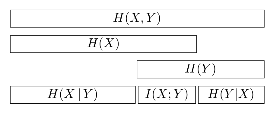
Mutual information overview.

Kullback-Leibler divergence

Let \(X\) be a random variable and \(p(x)\) and \(q(x)\) two probability distributions over this random variable. The Kullback-Leibler divergence is defined as

\[D_{KL}(p||q) = \sum_{x} p(x) \ log_2\left(\frac{p(x)}{q(x)}\right)\]

The Kullback-Leibler divergence is often called relative entropy and denotes “something” like a distance between two distributions:

\[\begin{split}&D_{KL}(p||q) \geq 0 \\ &D_{KL}(p||q) = 0 \iff p=q\end{split}\]

Yet it is not a real distance as symmetry is not given.

Typicality

We introduce the “Asymptotic equipartion” principle which can be seen as a law of large numbers. This principle denotes that for an ensemble of \(N\) independent and identically distributed (i.i.d.) random variables \(X^N \equiv (X_1, X_2, \dots, X_N)\), with \(N\) sufficiently large, the outcome \(x = (x_1, x_2, \dots , x_N)\) is almost certain to belong to a subset of \(\mathcal{A}_X^N\) with \(2^{NH(X)}\) members, each having a probability that is ‘close to’ \(2^{-NH(X)}\).

The typical set is defined as

\[T_{N \beta} \equiv \{ x \in \mathcal{A}_X^N : | \frac{1}{N} \log_2 \frac{1}{P(x)} - H | < \beta \}.\]

The parameter \(\beta\) sets how close the probability has to be to \(2^{-NH}\) in order to call an element part of the typical set, \(\mathcal{A}_X\) is the alphabet for an arbitrary ensemble \(X\).

Shannon’s Source Coding Theorem

Mathematical Terms in Tishby’s Experiments

Stochastic Gradient Descent

Spherical Harmonic power spectrum [Tishby (2017) 3.1 Experimental setup]

TODO

O(3) rotations of the sphere [Tishby (2017) 3.1 Experimental setup]

TODO