Background
An introduction to artificial neural networks
Making some sorts of artificial lives, capable of acting humanly-rational, has been a long lasting dream of mankind. We started with mechanical bodies, working solely based on laws of physics, which were mostly fun creatures rather than intelligent ones. The big leap took place as we stepped in the programmable computers era; when the focus shifted to those features of human skills which were a bit more brainy. So the results became more serious and successful. Codes started beating us in some aspects of intelligence which involve memory and speed, especially when they were tested using well, and formally, structured s. But their Achilles Heel was the tasks that need a bit of intuition and our banal common sense. So, while codes were instructed to outperform us at solving elegant logical problems at which our brains are miserably weak, they failed to carry out some simple trivial tasks that we are able to do, even without consciously thinking about them. It was like we made an intangible creature who is actually intelligent, but in a different direction perpendicular to the direction of our intelligence. Thus, we thought if we really want something that act similar to us, we need to structure it just like ourselves. And that was the very reason for all the efforts that finally led to the realization of artificial neural networks (ANNs).
Unlike the conventional codes, which are instructed what to do, in a step-by-step way and by a human supervisor, neural networks learn stuff by observing data. It is almost the same as the way our brain learns doing intuitive tasks that we have no clear idea of exactly how and exactly when we have learned doing them; for example, a trivial task like recognizing a fire hydrant in a picture of a random street. And that was the way we chose to tackle the common sense problem of AI. So, what are these neural networks?
Perceptron
Let’s start with the perceptron, which is a mathematical model of a single neuron and the plainest version of an artificial neural network: a network with one single-node layer. However, from a practical point of view, a perceptron is only a humble classifier that divide input data into two categories: the ones that cause our artificial neuron fires, and the ones that does not. The procedure is like this: the perceptron takes one or multiple real numbers as input, sums over a weighted version of them, adds a constant value, bias, to the result, and then uses it as the net input to its activation function. That is the function that calculates if the perceptron is going to be activated with the inputs or not. The perceptron uses Heaviside step function as its activation function. So the output of this function is the the perceptron output.

Fig. 1. Perceptron
In language of math, a perceptron is a simple equation:
Eq. 1
where xi is the ith input, wi is the weight correspond to the ith input, b stands for the bias, and H is the Heaviside step function which will be activated with positive input:
Eq. 2 [1]
For the sake of neatness of the equation, we add a facial input, x0 , which is always equal to 1 and its weight, w0 , represent the bias value. Then we can rewrite the perceptron equation as:
Eq. 3
and simplify the diagram, by removing the addition node, assuming everyone knows that the activation function will work on the summation of inputs:

Fig. 2. Perceptron
Hands On (1)
If we have [.5, 3, -7] as inputs, and [4, .2, 9] as our weights, and the bias sets to 2, the net
input to the Heaviside step function is:

4(.5)+.2(3)+9(-7)+2 = -58.4

And since the result is negative, the perceptron output is 0.
Snippet (1)
Perceptron could be easily coded. It is just a bunch of basic math operations and an if-else
statement. Here is an example code, using Python:
import numpy as np

def perceptron(input_vector):
    '''
    This perceptron function takes a 3-element
    array in form of a row vector as its argument,
    and returns the output of the above described
    perceptron.
    '''

    # setting the parameters
    bias = 2
    weights = np.array([4, .2, 9])

    # calculating the net input to the HSFunction
    input = np.inner(input_vector, weights) + bias

    # implementing Heaviside step function
    if input < 0:
        output = 0
    else:
        output = 1

    return output


input_vector = np.array([.5, 3, -7])
print('The perceptron output is ', perceptron(input_vector))
As we did with the code, dealing with a perceptron, the input is the only variable we have. But the weights and the bias are the parameters of our perceptron and parts of its architecture. It does not necessarily mean that the weights and the bias take constant values. On the contrary, we will see that the most important, and the beauty, of perceptron is its ability to learn and this learning happens through the change of the weights and the bias.
But for now, let’s just talk about what does each of the perceptron parameters do? We can use a simple example. Assume you want to use a perceptron deciding if a specific person likes watching a specific movie or not.[2] You could define an almost arbitrary set of criteria as your perceptron input, like the movie genre, how good are the actors, and say the movie production budget. We can quantize these three criteria assuming the person loves watching comedies, so if the movie genre is comedy (1) or not (0). And the total number of prestigious awards won by the four leading/supporting actors, and the budget in million USD. The output 0 means the person, probably, does not like the movie and 1 means she, probably, does.
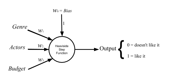
Fig. 3. A perceptron for binary classification of movies for a single Netflix user
Now it is easier to have an intuitive understanding of what each of perceptron parameters does. Weights help to give a more important factor, a heavier effect on the final decision. So for example, if the person is a huge fan of glorious fantasy movies with heavy CGI, we have to set w1 a little bit higher. Or if she is open to discovering new talents over watching the same arrogant acting styles, we could lower down w2 a bit. The bias role, however, is not as obvious as the weights. The simplest explanation is that bias shift the firing threshold of the perceptron or to be accurate the activation function. Suppose the intended person cares equally for the three elements of input and won’t watch a movie that fails to meet each one them. Then we have to set the bias so high that a high score in none of these three indices cannot make the perceptron fire, singly. Or if she probably would like Hobbit-kinds of movie, even though they do not fit in comedy genre, we can lower down the bias to the extent that having high scores, the Actors and the Budget could fire the perceptron together. You might think that we could do all these kind of arrangements solely using the weights. So let’s deal with this case in which all the input parameters are equal to zero. Without adding a bias term the output would be zero regardless of what we are taking in, and what we are willing to classify.
Hands On (2)
Assume we have two binary inputs, A and B, which could be either 0 or 1. What we want is to
design a perceptron that takes A and B and behaves like a NOR gate; that is the perceptron
output will be 1 if and only if both A and B are 0, otherwise the output will be 0.

It is not always guaranteed for all problems, but in this case, we could do the design in too
many different ways, with a wide variety of values as weights and the bias. One possible valid
combination of the parameters is: wA = -2, wB = -1, and the bias = 1. We can check the results:

Another valid set of parameters would be: wA = -0.5, wB = -0.5, and .4 for the bias. You can
think of many more sets of valid parameters yourself.

Now try designing this perceptron without adding bias.
The last thing to talk about is the activation function. The function is like the perceptron brain. Even though it does not do complicated calculations, but without it the perceptron is nothing but a linear combination of the inputs.[3] The activation function helps perceptron to learn. Once the perceptron parameters are set, it is able to differentiate between different sets of inputs and to make decisions via its elementary mechanism of ‘fire’ or ‘do not fire’.
That would be also fun to compare a perceptron with a neuron; provided that you do not take this comparison too seriously.[4] You can think of the inputs, naïvely, as chemoelectrical signals transmitting through dendrites (weights), reaching the neuron (Heaviside step function), if the pulse passes the threshold (bias), the neuron fires down the axon (the output is 1), otherwise it does not (the output is 0).
The Network
So… not a big deal? We have a basic classifier which it is limited to linearly separable data. Suppose we want to divide a set of samples that are, somehow, represented using a coordinate system. The perceptron would be able to do the task, if and only if, the two sets could be separated by drawing a single straight line between them.[5]
Problem (1)
Design a perceptron that takes two binary inputs, A and B and returns the XOR value of them:

So at this point, perceptron might seem a little boring. But we can make it wildly exciting with taking one step further in imitating our brain structure by connecting artificial neurons together to form a network in which each perceptron output is fed as input to another perceptron; something like this:
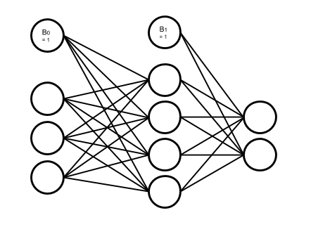
Fig. 4. An artificial neural network
As you see in the picture, the artificial neurons, or simply the nodes, are organized in layers. Nodes in a layer are not connected to each other. They are just connected to other nodes in their previous and/or next layers, except for the bias nodes. The bias nodes are not connected to their previous layer nodes, because being connected backward means their value is going to be set with the incoming flow. But bias nodes, as we see in perceptron, are conventionally set to feed 1,[6] so they are disconnected from their previous layers.
The first layer of the network is the input layer, and the last one is the output layer. Every layer in between is called a hidden layer. Note that, in the above picture, the input layer is more of a decorative setting, or a placeholder only to represent the input flow. The nodes in this layer are not actual perceptrons. They, just like the bias nodes, merely stand for input variables, and unlike the other nodes in the network, do not represent any activation function.[7] When we are counting a network layers, we only consider the layers with adjustable weights led to them. So in this case, we do not count the input layer and say it is a 2-layer neural network, or the depth of this network is 2. The number of neurons in each layer is called its width. But, just like the poor input layer, we do not include bias nodes while counting the width. So in our network the hidden layer width is 4 and the output layer width is 2.
As the depth of the network increases, it could easier deal with the more complicated patterns. The same happens when the width of layers grows. What this complex structure does is to break down the input data into small fragments and find a way to combine the most informative parts as output.
Imagine we want to estimate people income, based on their age, education, and say blood pressure. Assume we want to use the multiple linear regression method to accomplish the task. So what we do is to find how much and in which way each of our explanatory variables (i.e. age, education, and blood pressure) affects the income. That is, we reduce income to summation of our variables multiplied by their corresponding coefficient plus a bias term. Sounds good, does not work all the time. What we neglect here is the implicit relations between the explanatory variables, themselves. Like the general fact that, as people age, their blood pressure increases. Now what a neural network with its hidden layers does is to taking these relations into account. How? With chopping each input variable into pieces, thanks to many nodes in a one single layer, and letting these pieces each of which belongs to a different variable, combine together with a specific proportion, set by the weights, in the next layer. In other word, a neural network let the input variable have interaction with each other. And that is how the increase of width and the depth enable the network to handle and to construct more complex data structures.
Problem (2)
We discussed a privilege of neural networks over the multiple linear regression in doing a specific
task. Regarding the same task, would the neural network performance still have any privilege over a
multivariate nonlinear regression, which can handle nonlinear dependency of a variable on multiple
explanatory variables?
Snippet (2)
Assume we have the following network, in which all the nodes in the hidden and output layers have
Heaviside step function as their activation function:
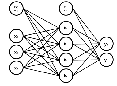
The hidden layer weights are given with the following connectivity matrix:
So according to this matrix, w32 or the weight between the second input x2 and the third node in the
hidden layer, h3, is 5. That is, x2 will be multiplied by -5, before being fed to h3. You might feel
a little uncomfortable with w32 convention of labeling and like w23 much better. But you will see
noting the destination layer index before the origin layer makes life much easier. In addition, you
can always remember that the weights are set only to adjust the value which is going to be fed to
the next layer.

And, in the same way, the following connectivity matrix gives us the output layer weights:
And the bias vectors are:
Now we want to write a code to model this network, get a numpy array with the shape of (3,) as the
input and returns the network output:
import numpy as np

# Modeling Heaviside Step function
def heaviside(z):
    '''
    This function models the Heaviside Step Function;
    it takes z, a real number, and returns 0 if it is
    a negative number, else returns 1.
    '''
    if z < 0:
        return 0
    else:
        return 1

# And vectorizing it, suitable for applying element-wise
heaviside_vec = np.vectorize(heaviside)

def ann(input_0):
    '''
    This Artificial Neural Network function takes a 3-element
    array in the form of a row vector as its argument, and returns
    a two-element row vector as its output.
    '''

    # setting the parameters
    bias_0 = np.array([2, -3, 1, .6])
    bias_1 = np.array([4, 5])
    weights_10 = np.array([[4, 3, 2], [-2, 1, .5], [2, -5, 1.2], [3, -1, 6]])
    weights_21 = np.array([[2, -1, 5, 3.2], [-4.5, 1, 3, 2]])

    # calculating the net input to the first (hidden) layer
    input_1 = np.matmul(weights_10, input_0.transpose()) + bias_0.transpose()

    # calculating the output of the first (hidden) layer
    output_1 = heaviside_vec(input_1)

    # calculating the net input to the second (output) layer
    input_2 = np.matmul(weights_21, output_1.transpose()) + bias_1.transpose()

    # calculating the output of to the second (output) layer
    output_2 = heaviside_vec(input_2)

    return output_2
So, now that we know the magic of more nodes in each layer and more hidden layers, what does stop us from voraciously extending our network? First of all we have to know that it is theoretically proven that a neural network with only one hidden layer can model any arbitrary function as accurate as you want, provided that you add enough nodes to that hidden layer.[8] However, adding more hidden layers makes life easier, both for you and your network. Then again, what is the main reason for sticking to the smallest network that would handle our problem?
With the perceptron, for example when we wanted to model a logic gate, it was a simple and almost intuitive task to find proper weights and bias. But as we mentioned before that the most important, and the beauty of a perceptron is its capacity to learn functions, without us setting the right weights and biases. It can even go further, and map inputs to desired outputs with finding and observing patterns in data that are hidden to our defective human intuition. And that is where the magical power of neural networks come from. Artificial neurons go through a trial and error process to find the most effective values as their weights and biases, regarding what they are fed and what they are supposed to return. This process takes time and would also be computationally expensive.[9] Therefore, the bigger the network, the slower and more expensive its performance. And that is the reason for being thrifty in implementing more nodes and layers in our network.
Activation Functions
Speaking of learning, how does perceptron learn? Assume that we have a dataset including samples with attributes a, b, and c. And we want to be able to train the perceptron to predict attribute c provided a and b. What the perceptron does it to start with random weights and bias. It takes the samples attributes a and b as its input and calculates the output, which is supposed to be the attribute c. Then it compares its result with the actual c, measures the error and based on the difference, it adjusts its parameters a little bit. The procedure will be repeated until the error shrinks to a desired neglectable level.
Cool! Everything seems quiet perfect, except the fact that the output of perceptron activation function is either 1 or 0. So if the perceptron parameters change a bit, its output does not change slowly, but jumps to the other possible value. Thus, the error is either at its maximum or minimum level. For making an artificial neuron trainable, we started using other functions as activation functions; functions which are, somehow, smoothed approximations of the original step function.
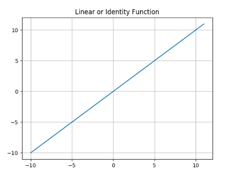
Linear or Identity Function
Earlier we talked about the absurdity of a perceptron (not to mention a network) not using an activation function, because its output would simply be a linear combination of the inputs. But, actually, there is a thing as linear or identity activation function. Imagine a network in which all nodes work with linear functions. In this case, according to linearity math, no matter how big or how elaborately-structured that network is, you can simply compress it to one single layer. However, a linear activation function could still be used in a network, if we use it as activation function of a few nodes; especially the ones in the output layer. There are cases, when we are interested in regression problems rather than classification ones, in which we want our network to have an unbounded and continuous range of outputs. Let’s return to example where we wanted to design a perceptron capable of predicting if a user wants to watch a movie or not. That was a classification problem because our desired range of output was discrete; a simple bit of 0 or 1 was enough for our purpose. But assume the same perceptron with the same inputs is supposed to predict the box office revenue. That would be a regression problem because our desired range of output is a continuous one. In such a case a linear activation function in the output layer would send out whatever it takes in, without confining it within a narrow and discrete range.
Eq. 4
Snippet (3)
Modeling the linear or identity activation function and plotting its graph:
import numpy as np
import matplotlib.pyplot as plt

def linear(z):
    '''
    This function models the Linear or Identity
    activation function.
    '''
    y = [component for component in z]
    return y


# Plotting the graph of the function for an input range
# from -10 to 10 with step size .01

z = np.arange(-10, 11, .01)
y = linear(z)

plt.title('Linear or Identity Function')
plt.grid()
plt.plot(z, y)
plt.show()
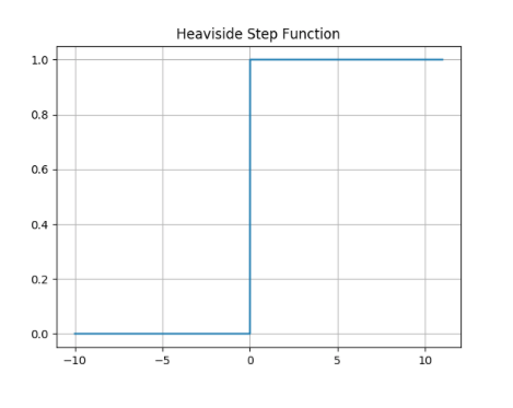
Heaviside Step Function
We already met the Heaviside step function:
Eq. 5
Snippet (4)
Modeling the Heaviside step activation function and plotting its graph:
import numpy as np
import matplotlib.pyplot as plt

def heaviside(z):
    '''
    This function models the Heaviside step
    activation function.
    '''
    y = [0 if component < 0 else 1 for component in z]
    return y


# Setting up the domain (horizontal axis) from -10 to 10
# with step size .01

z = np.arange(-10, 11, .01)
y = heaviside(z)

plt.title('Heaviside Step Function')
plt.grid()
plt.plot(z, y)
plt.show()
Sigmoid or Logistic Function
Sigmoid or logistic function is currently one of the most used activation functions, capable of being used in both hidden and output layers. It is a continuous and smoothly-changing function, and that makes it a popular option because these features let the neurons to tune its parameters at the finest level.
Eq. 6
Snippet (5)
Modeling the Sigmoid or Logistic activation function and plotting its graph:
import numpy as np
import matplotlib.pyplot as plt

def sigmoid(z):
    '''
    This function models the Sigmoid or Logistic
    activation function.
    '''
    y = [1 / (1 + np.exp(-component)) for component in z]
    return y


# Plotting the graph of the function for an input range
# from -10 to 10 with step size .01

z = np.arange(-10, 11, .01)
y = sigmoid(z)

plt.title('Sigmoid or Logistic Function')
plt.grid()
plt.plot(z, y)
plt.show()

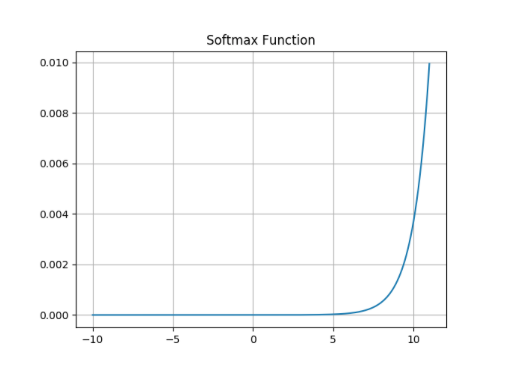
Softmax Function
Let’s go back to the movie preferences example. In the original problem setting, what we wanted to do was to know if the user likes watching a specific movie or not. So our desired output was a binary classification. Now consider a situation when we also want to check the user interest in movie using multiple level; for example: she does not like to watch the movie, she likes to watch the movie, she likes the movie so much that she would purchase the first video game produced based on the movie. And instead of a decisive answer of 0 or 1, we want a probability value for each of these three outcomes, in a way that they sum up to 1.
In this case, we cannot use a sigmoid activation function in the output layer anymore; even though the sigmoid neurons output works well as probability value, but it only handle binary classifications. Then that is exactly when we use a Softmax activation function instead; that is, when we want to do a classification task with multiple possible classes. You can think of Softmax as a cap over your network multiple, and raw, outputs, which takes them all and translates the results to a probabilistic language.
Since Softmax is designed for such a specific task, using it in hidden layers is irrelevant. In addition, as you will see in the equation, what Softmax does is to take multiple values and deliver a correlated version of them. The output values of a Softmax node are dependent on each other. That is not what we want to do with our raw stream of information in our neural network. We do not want to constrain the information flow in the network, in any possible way, when we do not have any logical reason for that. However, recently, some researchers have found a good bunch of these logical reasons to use Softmax in hidden layers.[10] But the general rule is do not use it in hidden layer as long as you do not have a clear idea of why you are doing this.[11] Anyway, this is the Softmax activation function:
Eq. 7
To have a better understanding of what is going on over there, the following diagram could be useful:

Fig. 5. Softmax layer
Snippet (6)
Modeling the Softmax activation function and plotting its graph:
import numpy as np
import matplotlib.pyplot as plt

def softmax(z):
    '''
    This function models the Softmax activation function.
    '''
    y = [np.exp(component) / sum(np.exp(z)) for component in z]
    return y


# Plotting the graph of the function for an input range
# from -10 to 10 with step size .01

z = np.arange(-10, 11, .01)
y = softmax(z)

plt.title('Softmax Function')
plt.grid()
plt.plot(z, y)
plt.show()
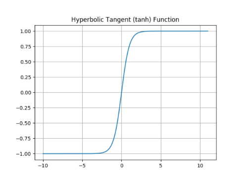
Hyperbolic Tangent or TanH Function
Hyperbolic tangent activation function or simply tanh is pretty much like the sigmoid function, with the same popularity, and the same s-like graph. In fact, as you can check with the equation, you can define the tanh function using a horizontally and vertically, scaled and shifted version of the sigmoid function. And for that reason you can model a network with tanh hidden nodes using a network with sigmoid hidden nodes and vice versa. However, unlike the sigmoid function which its output is between 0 and 1, and therefore a lovely choice for probabilistics problems, tanh output ranges between -1 and 1, and therefore is zero centered, thanks to the vertical shift we mentioned. That enables tanh function to handle negative values with its negative range. For the very same reason, training process is easier and faster with tanh nodes.
Eq. 8
Snippet (7)
Modeling the tanh activation function and plotting its graph:
import numpy as np
import matplotlib.pyplot as plt

def tanh(z):
  '''
  This function models the Hyperbolic Tangent
  activation function.
  '''
  y = [np.tanh(component) for component in z]
  return y

# Plotting the graph of the function for an input range
# from -10 to 10 with step size .01

z = np.arange(-10, 11, .01)
y = tanh(z)

plt.title('Hyperbolic Tangent (tanh) Function')
plt.grid()
plt.plot(z, y)
plt.show()
Rectified Linear Unit or ReLU Function
Rectified Linear Unit or ReLU function, currently, is the hottest activation function in the hidden layers. Mathematically, ReLU is the step function and linear function joining together at the point zero. It rectifies the linear function by shutting it down in negative range.
Eq. 9
This combination makes it benefit from the good features of both functions. That is, while ReLU enjoys the unboundness of linear function, thanks to its behavior in the negative range, it is still a nonlinear function, not a barely, hardly useful linear function. We discussed that no matter how deep and how complex is a network of linear nodes, you can compress it to a single layer network of the same linear nodes. On the other hand, a network formed of ReLU neurons, could model any function you think of. The reason is that the nonlinearity of ReLU function will be chopped into random pieces and combined in complex patterns going through hidden layers and neurons; just the same as what happens to information flow in a neural network. And that makes the network nonlinear with a desirable level of complexity. In addition, ReLU benefits its linear part the way that the linear function itself can barely make use of. As we mentioned training a network needs a steady and slow rates of change in the network output. A feature that is missing in sigmoid and tanh neurons when we move towards big negatives and positives value. At those ranges, sigmoid and tanh have asymptotic behavior which means their change rates get undesirably slow and diminish. But ReLU has a steady rate of change, albeit for the positive range. There is one more beautiful thing about ReLU behavior in negative range. Networks with sigmoid and tanh neurons are firing all the time; but a ReLU neuron just like its wet counterpart sometimes does not fire, even in the presence of a stimuli. So using ReLU we can have sparse activation networks. This property, alongside with the steady rate of change, and its simple form, enables ReLU not only to have a faster training session, but also to be computationally less expensive. Though this negative blindness of ReLU has its own issues, as well. First and most obvious, it cannot handle negative values. Secondly, we have this problem called dying ReLu, that happens in the negative range, when the rate of change becomes zero. So when a neuron produce a big enough negative output, changing its weights and bias does not show any regress or progress; just like a dead body sending out flatline.
Snippet (8)
Modeling the ReLU activation function and plotting its graph:
import numpy as np
import matplotlib.pyplot as plt

def relu(z):
    '''
    This function models the Rectified Linear Unit
    activation function.
    '''
    y = [max(0, component) for component in z]
    return y

# Plotting the graph of the function for an input range
# from -10 to 10 with step size .01

z = np.arange(-10, 11, .01)
y = relu(z)

plt.title('Rectified Linear Unit (ReLU) Function')
plt.grid()
plt.plot(z, y)
plt.show()

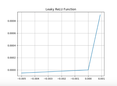
Leaky ReLU Function
And the Leaky ReLU function is here to solve the negative issues about the negative blindness of ReLU function aka dying ReLU. So instead of a flatline with zero change rate, leaky ReLU leaks a little in negative range, with an arbitrary, but gentle slope, usually set to .01. But it costs us the ‘sparse activation’ advantage of ReLU.
Eq. 10
Snippet (9)
Modeling the Leaky ReLU activation function and plotting its graph:
import numpy as np
import matplotlib.pyplot as plt

def lRelu(z):
  '''
  This function models the Leaky ReLU
  activation function.
  '''
  y = [max(.01 * component, component) for component in z]
  return y

# Plotting the graph of the function for an input range
# from -.005 to .001 with step size .001

z = np.arange(-.005, .001, .001)
y = lRelu(z)

plt.title('Leaky ReLU Function')
plt.grid()
plt.plot(z, y)
plt.show()
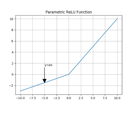
Parametric ReLU or PReLU Function
Parametric ReLU or PReLU function is a variant of the Leaky ReLU, in that the slope is not constant but it is defined as a another parameter of the network, 𝛼, which will be tuned during training just like other parameters, weights and biases.
Eq. 11
Snippet (10)
Modeling the PReLU activation function and plotting its graph:
import numpy as np
import matplotlib.pyplot as plt

def pRelu(z):
  '''
  This function models the Parametric ReLU or PReLU
  activation function with alpha equals to .3.
  '''
  y = [max(.3 * component, component) for component in z]
  return y

# Plotting the graph of the function for an input range
# from -10 to 10 with step size .01

z = np.arange(-10, 10, .01)
y = pRelu(z)

plt.title('Parametric ReLU Function')
plt.annotate(r'y=$\alpha$x', xy=(-5, -1.5), xytext=(-5, 1.5),
            arrowprops=dict(facecolor='black', width=.2))
plt.grid()
plt.plot(z, y)
plt.show()
Maxout Function
You see how PReLU was generalizing Leaky ReLU, and Leaky ReLU was, somehow, generalization of ReLU. Now, the Maxout activation function is a big step further in generalization of ReLU family of activation functions. Think about PReLU one more time, and this time try to see it as a combination of two linear functions.
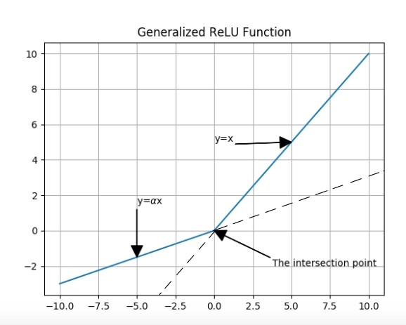
Fig. 6.
So, what ReLU family do, basically, is to take the x and compute the corresponding y, using two lines’ equations, and then pass the biggest y as the output. Now, what Maxout does, is to do the same except two things. First, Maxout won’t limit itself to only two lines. And second, those lines that Maxout work with, do not have pre-defined equations, but their characteristics like slope and y-insects will be learned. From this aspect, you can say Maxout is not just training the network, but on a lower level, it is also training the activation function, itself.

Fig. 7.
Maxout has a two-stage mechanism. There are linear nodes, at the first stage, which take the previous layer outputs (or the networks input, for sure) as their inputs, and the next stage is just a simple function, picking the maximum out.
Eq. 12
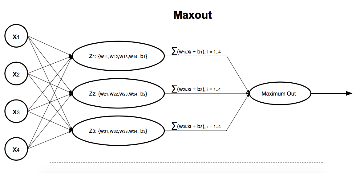
Fig. 8. Maxout inside workings
In the above picture, we have a Maxout neurons with 3 linear nodes. As you might noticed, Maxout linear nodes will be fed with net outputs of the previous layer (or network inputs), instead of being processed by weights and biases. The reason is obvious; Maxout weights and biases are shifted to its linear nodes. A network with two Maxout neurons can approximate any continuous function with an arbitrary level of accuracy.
Snippet (11)
Modeling the Maxout activation function:
import numpy as np
import matplotlib.pyplot as plt

def maxout(x, w, b):
  '''
  This function models the Maxout activation function.
  It takes input, x, the Maxout linear nodes weights, w,
  and its biases, b, all with numpy array format.
  x.shape = (1,i)
  w.shape = (n,i)
  b.shape = (1,n)
  i = the number of Maxout inputs
  n = the number of Maxout's linear nodes
  '''
  y = np.max(w @ np.transpose(x) + np.transpose(b))
  return y
Exponential Linear Unit or ELU Function
Softplus Function
Radial Basis Function
Swish Function
Arctangent Function
Hard Tangent Function
Problem (3)
Think of a new activation function with some advantages over the popular ones. Run an expriment to
compare its perfocrmance with the others. If it outperforms the hot ones, publish a paper on it.

Statistical Dependence
If a random variable, called X, could give any information about another random variable, say Y, we consider them dependent. The dependency of two random variables means knowing the state of one will affect the probability of the possible states of the other one. In the same way, the dependency of a random variable could be passed and also defined for a probability distribution. Investigating a possible dependency between two random variables is a difficult task. A more specific and more difficult task is to determine the level of that dependency. There are two main categories of techniques for measuring statistical dependency between two random variables. The first category mainly deals with the linear dependency and includes basic techniques like the Pearson Correlation and the Spearman’s Measure. But these techniques do not have a good performance measuring nonlinear dependencies which are more frequent in data. The second category, however, include general techniques that cover nonlinear dependencies, as well.
1. Distance Correlation
Distance correlation (dCor) is a nonlinear dependence measure and it can handle random variables with arbitrary dimensions. Not surprisingly, dCor works with the distance; the Euclidean distance. Assume we have two random variables X and Y. The first step is to form their corresponding transformed matrices, TMx and TMy. Then we calculate the distance covariance:
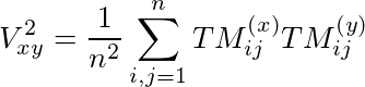
And finally, we calculate the squared dCor value as follows:

The dCor value is a real number between 0 and 1 (inclusively), and 0 means that the two variables are independent.
2. Mutual Information
Mutual information (MI) is a general measure of dependance based on the core concept of information theory, ‘entropy.’ Entropy is a measure of uncertainty, and is formulated based on the average ‘information content’ of a set of possible outcomes of an event, which is in turn, a measure of information.
Information content of the outcome x with probability P(x):

Entropy of an event with N outcomes with probabilities P1…Pn:

Mutual information is a symmetric relation between two variables and it indicates the amount of information that one random variable reveals about the other. Or in other words the reduction of uncertainty about a variable, resulted from our knowledge about another one:
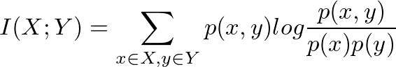
Mutual information is a symmetric and non negative value. And a zero MI means two independent variables.
Calculating MI for discrete valued variables is somewhat easy, the problem arises when we try to calculate MI, or in fact the entropy itself, for variables with real, continuous values. For working under this condition, we use the other version of MI formula which is a specific form of the more general form of Kullback-Leibler divergence and works on Probability Density Function (PDF) of joint probabilities:

However, the need for knowing PDF is another problem. In practice, we usually have access to a finite set of data spamles, and not the PDF they are representing. So before being able to calculate MI, or in essence entropy, we need to approximate the PDF itself. In this sense, the problem of estimating MI reduces to the problem of estimating PDF. In fact, most of MI estimators start with PDF estimation procedure. There are two main groups of MI estimators: parametric and non-parametric estimators. Parametric estimators are the ones that assume the probability density could be modelled with one of the most frequent distributions like Gaussian. Non-parametric estimators assume nothing about the hidden PDF.
The main approaches for estimating MI, in a non-parametric way, are methods based on histogram, adaptive partitioning, kernel density, B-spline, and k-nearest neighbor.
2.1. Histogram-based Estimation
Using a histogram is a simple, neat, and popular approach for MI estimation, which is computationally easy and efficient: we discretize the distribution into N number of bins, count the number of occurrences of samples per bin. The number of bins is an arbitrary option, best decided on, cosidering the nature of our data. Using bins with constant width make our estimation too sensitivie to the that arbitrary number of N which could lead ignoring some meaningful patterns in our data, only because some samples were interpreted within two neighboring, instead of one single bin. That is, constant bins number or their width is not sensitive to the changes in data stream, and therfore, not as efficient as the histogram estimation could potentially be. So another way is to focus on the bins width rather than their number and try to define them variably. This approach will reduce the estimation error, but would increase the complexity of the computation by adding a new problem of how to decide about the changing bin-width and how to implement the decision.
An example of using histogram estimation. Haeri, M. A., & Ebadzadeh, M. M. (2014). Estimation of mutual information by the fuzzy histogram. Fuzzy Optimization and Decision Making, 13(3), 287-318.
2.2. Adaptive Partitioning
Adaptive partitioning, as it is clear from its name, is another way of dividing data space into subsets and subsequent counting of the covered occurrences. The new thing about adaptive partitioning is that it does not confine itself to classic histogram bins, rather it feels free to use different-sized rectangular tiles to cover the data space in a way that increase the conditional independence between partitions. Partitioning is done through an iterative procedure in which after each step, the conditional independence of each tile regarding the other partitions will be examined using Chi-square statistical test.
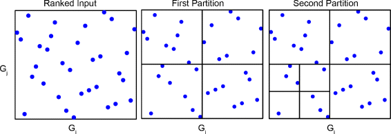
An example of adaptive partitioning procedure. He, J., Zhou, Z., Reed, M., & Califano, A. (2017). Accelerated parallel algorithm for gene network reverse engineering. BMC systems biology, 11(4), 83.
2.3. Kernel Density Estimation (KDE)
Kernel density estimation, outperforms both histogram and adaptive partitioning methods, in accuracy. But, not surprisingly, it is computationally a heavier and slower method. The main difference and advantage of KDE is its tolerance in partitioning. KDE not only does not restrict itself to rectangular, so to say, bins or any specific point in data space as the origin, and it also does not use strict lines at borders. What it uses is a kernel with an arbitrary width. This arbitrariness, again, is a weakness and makes the resulted PDF sensitive to the decision on the kernel width. In the next step, KDE calculates one of different possible probability densities including Gaussian, Rectangular, and Epanechnikov around each data samples, add them up together to obtain a smooth PDF over all data samples from the superposition of these kernels. The resulted PDF is of high quality because of a smaller MSE rate.
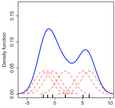
Implementing KDE. http://daveakshat.blogspot.com/2013/04/convolution-probabilty-density.html
2.4. B-Spline
This method is simply using basis spline function to approximate the underlying PDF. A B-spline function separates dataspce with equally-distanced hypotetical lines (or thier counterparts in case of working with higer dimensional data) and try to regress the data points trapped in each interval with a polynomial function. These continuous functions form the PDF which we will use later for calculating MI. B-spline results usually improve by increasing the function order. But when the final goal is estimating MI, increasing the order to more than 3 won’t affect the result.
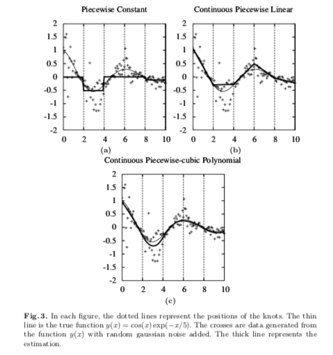
An example of using splines with different orders to approximate an underlying function. Venelli, A. (2010, April). Efficient entropy estimation for mutual information analysis using B-splines. In IFIP International Workshop on Information Security Theory and Practices (pp. 17-30). Springer, Berlin, Heidelberg.
2.5. K-Nearest Neighbor (KNN)
K-Nearest Neighbor method has a big difference with the previous MI estimators. It bypasses the PDF approximation phase and jumps right into the MI calculation phase. There is a family of KNN-based method for estimating MI, but the most popular one is the KSG. KSG uses a slightly modified MI formula in which the marginal and joint entropies for each data sample for each of two random variables are calculated using KL entropy estimator. KL entropy estimator computes entropy based on KNN idea, and with regards to the K smallest distances in a data set. KSG results are of high precision and it is a great option while working with high dimensional data. KSG is capable of working with irregular PDFs and it, currently, is one of the most popular MI estimators.

The pseudocode for KSG. Gao, W., Kannan, S., Oh, S., & Viswanath, P. (2017). Estimating mutual information for discrete-continuous mixtures. In Advances in Neural Information Processing Systems (pp. 5986-5997).
How does ‘Statistical Dependance’ help understanding deep learning?
Artificial neural networks were originaly designed to somehow replicate our biological neural network. Researcher were also partially hopeful to be able, by this replication, to learn a thing or two about the inner workings of human brain. But the irony is that the ANNs, especially the ‘deep neural network’ generation, turned to such a successful computational structure that its excellent behavior became a mysterious puzzle itself.
Publishing three papers in 1999, 2015, and 2017, Tishby offered and explored an idea for demystifying the DNN excellency using information theory concepts. According to Tishby, the key feature of a DNN is its capacity to forget. It is crucial to forget because not all the input information is necessary for accomplishing the task at the output layer. For example, consider a classification task in which pictures of cats and dogs are fed into the network and the network should decide whether an input image represent a cat or a dog. Feeding a cat photo into the network, we enter not only information about the shape of the animal but also its color. However, we know that whatever color is the animal, it does not affect its catish nature. For good results, the network should recognize and focus on the, probably the animal ear shape or face structure. So there is lots of information available which not only consume computational efforts, but also might mislead a network in its final decision. So what is important here, is not the ‘information,’ rather the ‘relevant’ information. That is where the ‘forgetting’ thing seems essential.
To make his point, Tishby offers his readers a Markov-chain perspective of a DNN and then tries to assess how the information flow is traveling through the DNN layers. For proving his theory of forgetting irrelevant data, he needed to show that the information flow in each layer leaves behind some parts of the input content and becomes more similar to the information content of the desired labels. Tishby calls this procedure ‘successive refinement of relevant information’. For doing so, he made use of mutual information concept. The mutual information between each layer and the input/labels was calculated using a histogram estimator with constant and equally-spaced bin size.
Tishby, then, defined a new plot for representing the information flow in a deep network, called ‘information plane.’ The x-axis of the information plane corresponds to I(X;T) which is mutual information between the input and the hidden layers. The y-axis corresponds to I(T;Y) which is mutual information between the hidden layers and the labels. In simple words, the horizontal axis tells us how much information a specific hidden layer is conveying about the input data and the vertical axis tells us how much information a specific hidden layer is conveying about the labels.
What Tishby seems to find out through his information plane was dazzling:

https://www.quantamagazine.org/new-theory-cracks-open-the-black-box-of-deep-learning-20170921/
|
|
The information plane shows a really interesting path of information flow or in fact mutual information ratio, especially, in the last hidden layers of DNN. It seems like the last layers start with a very low mutual information with the input data which is understandable, because the input data passing through all the layers with all their neurons had enough time to scattered enough not to be statistically similar/dependance to the original data at the input layer. So, these layers start with low I(X;T) but spend training time to gather enough information and generalize the ‘concepts’ in the input data. Tishby called this phase of increasing I(X;T) ‘fitting phase.’
Then, as you see, the last hidden layers start to lose input information, but at the same time gain information, or in fact structures of information, similar to the labels data. So their I(T;Y) keep increasing while I(X;T) is decreasing. Tishby calls this phase, ‘compression phase,’ in which the network lose irrelevant data and compress its information flow. And according to Tishby, this phase change and ‘forgetting’ process is what makes the deep learning so efficient and successful.
| [1] | We usually denote an activation function input with the letter z, rather than good old x, in order to prevent any confusion of the function input with the perceptron/network inputs. |
| [2] | For motivation, assume Netflix offered a US$1,000,000 prize for designing this perceptron. |
| [3] | Plus bias which in no-activation-function case, is itself an irrelevant factor. |
| [4] | Yes, the original idea was to imitate the way our brain works, but let’s be honest with ourselves, do we know how our brain works? But that aside, perceptron and ANNs have adopted a couple of important and effective macro features of our brain structure, like not being a simple/linear transmitter but getting activated with specific functions/patterns or the network structure itself which is made up of, generally, uniform elements. |
| [5] | Or a plane/hyperplane for 3 and more dimensions. |
| [6] | The value 1 is arbitrary, and only more convenient to work with. But whatever other value you assign to the bias nodes it should be constant during the flow of data through the network. |
| [7] | However, we will see that this is not a rule. |
| [8] | And provided that the nodes’ activation functions are nonlinear. |
| [9] | Both in an abstract and also a physical sense. |
| [10] | Xu, K., Ba, J., Kiros, R., Cho, K., Courville, A., Salakhudinov, R., … & Bengio, Y. (2015, June). Show, attend and tell: Neural image caption generation with visual attention. In International conference on machine learning (pp. 2048-2057). |
| [11] | Compare with the fact that you can use, say, a sigmoid neuron, almost wherever in a network that you want, without being sure of what you are doing! |