Measuring “Information”
The aim of the Information Bottleneck Theory is to understand the learning process in an ANN in information theoretical terms, that is from a more symbolic point of view. For that it is important to adopt the following view: Each layer is a representation of the layer before and thus a representation of the input. With this in mind it would be interesting to see how “information” flows through these representations, e.g. how much information does a hidden layer contain about the input. The big question that remains is: How do we measure this “information” and what do we actually mean with “information”?
Mutual information
Tishby identifies this “information” with the mutual information. As explained in earlier chapters mutual information is a measurement to describe how much uncertainty remains in a random variable if another dependent random variable is observed. The definition is
To understand how “information” flows through the graph Tishby proposed to look at the mutual information of each hidden layer \(T\) with the input \(X\) and with the label \(Y\).
Estimating Continuous entropy
If the dataset is continuous, like most datasets are, and the corresponding probability distribution is not available, like it is most of the time, you try to estimate the continuous entropy from the data you have. For this there are two algorithms that we looked into and we will shortly discuss.
The Estimator from Kolchinsky & Tracey (CITE PAPER)
This estimator does not estimate the entropy directly, but gives a upper and a lower bound. First we derive these estimator for a general probability distribution, which can be expressed as a mixture distribution
Now imagine drawing a sample from \(p_X\). This is equivalent to first drawing a \(c_i\) and then drawing a sample from the corresponding \(p_i(x)\).
For such a mixture distribution it can be shown that
The estimators will build on the notion of a premetric, which is defined the following way: A function \(D(p_i||p_j)\), which is always non-negative and is zero if \(p_i = p_j\) is called a premetric. With the help of premetrics we can define a general estimator for entropy:
for which it can be shown that it lies within the same bounds as the “real” entropy of a mixture distribution. The paper now shows empirically that we can get a good upper and lower bound by using the following two premetrics:
Upper bound: Kullback-Leibler divergence
Lower bound: Bhattacharyya distance
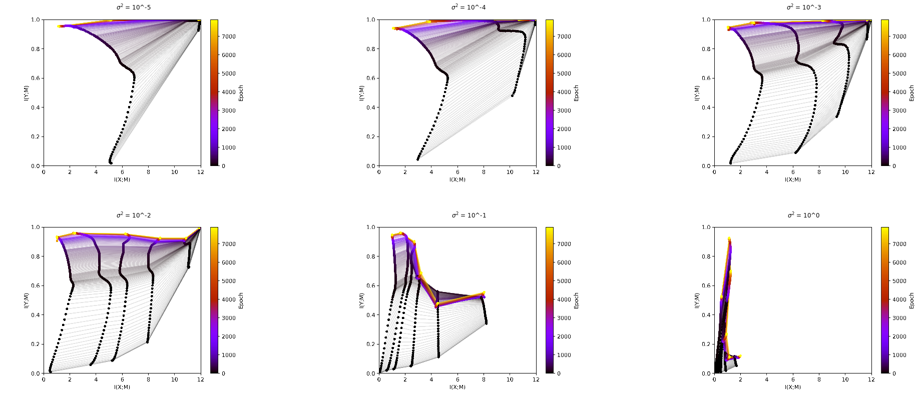
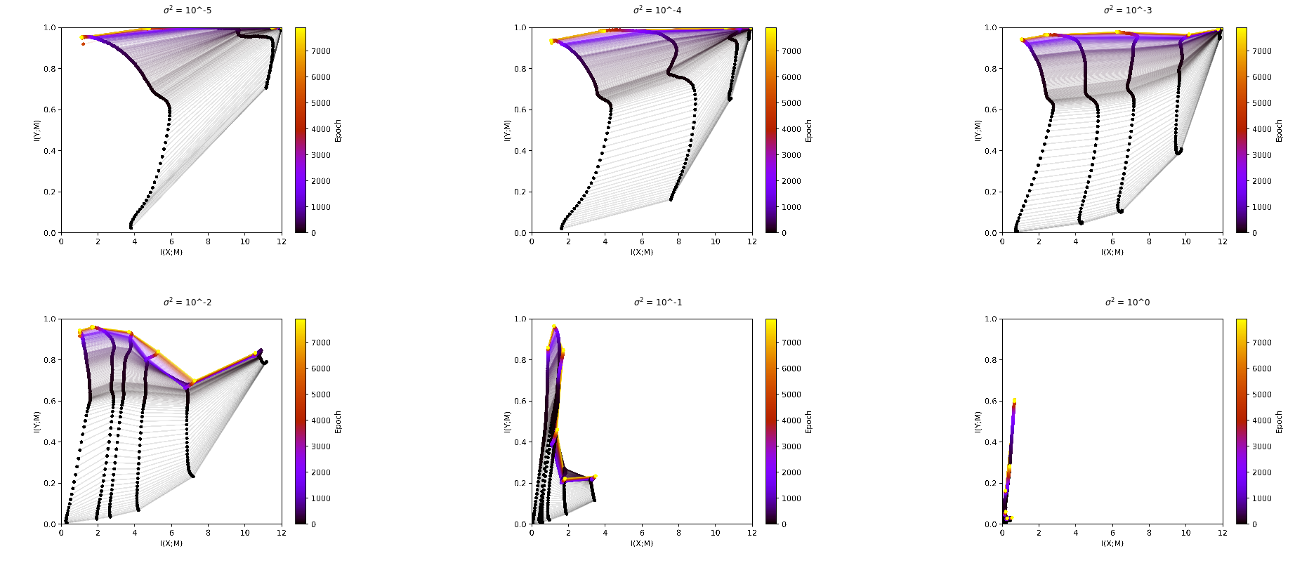
Now the question is how we use these estimators for mixture distributions in our case for estimating the entropy in a hidden layer of a neural network. We use the following trick: we look at our dataset as a mixture of delta functions. Accordingly our activations in a hidden layer can also be looked at as a mixture of delta functions. Doing this would give us an infinite mutual information between the input and the hidden layer though, so for purpose of analysis we have to add noise to the hidden layer. If \(h\) is the activation in the hidden layer we now define
This gives us now a mixture of gaussians with each gaussian centred at an activation corresponding to an input. In the following plots we can see that the \(\sigma^2\) we define when adding the noise is a free parameter which heavily influences the outcome.
The Estimator from Kraskov (CITE PAPER)
Discrete Entropy
The other option to continuous entropy would be discrete entropy, which is less mysterious and way easier to calculate. The problem is that for calculating discrete entropy we need discrete states. At this point it is interesting to note that the activations of a hidden layer are only continuous in theory. In practice they are restricted to the set of float32 values in each neuron, which would give you discrete states. If you use these states to calculate the entropy you get no difference in the mutual information over the different layers, as two different activations will nearly never be mapped to the exact same activation in the next layer. You can see this already for small binsizes like \(10^{-5}\) (see PLOT).
Binning
What Tishby did to solve this problem is to make the range, in which we say that two activations are the same bigger. This is what he calls binning. To define a binning you need to define either the number of bins or the size of bins you want. You could also define an upper and lower border, but it might make sense to take the highest and the lowest activation as the borders. The problem now is that this free parameter of the binsizes heavily influences the outcome.
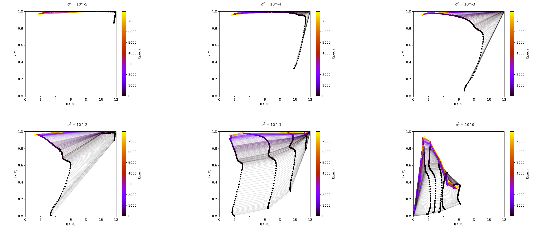
It is interesting to note here that the free parameter in the estimator from Kolchinsky & Tracey influences the plots in a very similar manner like the binsize.
Violation of the DPI
In the plot above you can see interesting behavior in the plots ???. You can see that later layers have more mutual information with the input then earlier layers. This is a violation of the data processing inequality, which states that information can only get lost but not created during processing of the data. If we look at a markov process
it should hold that \(I(X;h_1) \geq I(X;h_2)\) But this fact is easily explainable by the way we measure the information. Through the process of binning we are adding essentially some noise. But this noise is only added during the analysis and not during the training. So the DPI is violated here.