Effect of weight renormalization on activity patterns
In this experiment we show the influence of weight renormalization on the structure of activations in different layers.
Over the course of training the weights in a neural network usually get
larger. For tanh activated neurons as an example this means that on
average the preactivations will be larger in magnitude and therefore the
output of the neurons be close to either -1 or 1.
It was argued in the opposing paper that in general double-sided
saturating nonlinearities like tanh yield a compression phase as
neural activations enter the saturation regime. For relu, the
process of ever growing weights yields bigger activations over time for
the positive side of the activation spectrum. It is argued, that as
relu is not bounded for positive preactivations, this does not lead
to compression in later stages of the training.
Experiments with max_weight_norm=0.8
Here, we are picking up on these ideas by introducing rescaling of the weights after each epoch, such that the norm of every neuron’s weight vector does not exceed a specific threshold. We observe activation patterns that appear under these constraint during training and interpret these with respect to the phenomenon of “compression” in the infoplane plot.
In [1]:
import sys
sys.path.append('../..')
from deep_bottleneck.eval_tools.experiment_loader import ExperimentLoader
from deep_bottleneck.eval_tools.utils import format_config, find_differing_config_keys
import matplotlib.pyplot as plt
from io import BytesIO

import pandas as pd
import numpy as np
In [2]:
loader = ExperimentLoader()
In [3]:
experiment_ids = [599, 600, 601, 602]
experiments = loader.find_by_ids(experiment_ids)
differing_config_keys = find_differing_config_keys(experiments)
We first look at the informationplane plot for 4 different experiments.
We varied the activation function between tanh and relu as well
as fixing the maximum magnitude of the weight vector per neuron to 0.8
(max_norm_weights=0.8) or leaving the weight magnitude unconstrained
(max_norm_weight=False). The corresponding informationplane plots
for one run are displayed below.
In [4]:
fig, ax = plt.subplots(2,2, figsize=(16, 14))
ax = ax.flat

for i, experiment in enumerate(experiments):
    img = plt.imread(BytesIO(experiment.artifacts['infoplane'].content))
    ax[i].axis('off')
    ax[i].imshow(img)
    ax[i].set_title(format_config(experiment.config, *differing_config_keys),
                    fontsize=16)
plt.tight_layout()
plt.show()
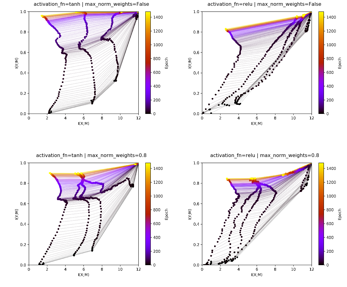
With no weight regularzation, for relu we see a pattern in the
infoplane as it has been reported before by the opposing paper. Except
for the last layer, which always has a softmax activation function,
no distict compression phase is visible. For tanh, the 5th layer
starts to compress, while all previous layers do not show distinct
compression. In a previously run experiment with several runs it was
comfirmed that on average over several runs the earlier layers do show
compression as well. Still, we keep in mind that the phenomenon is not
as stable as it might be suggested by reports of Tishby et. al.
Additionally, the prominent “dip” to the left after 60-100 epochs is
missing interpretation by previous works of Tishby and the opposing
paper. Also, it seems to be to consistent in some experimental settings
as to be only a result of random fluctuations.
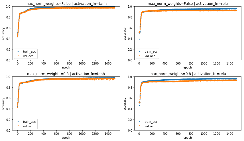
With weight normalization, several layers of tanh start to compress.
Furthermore and noteably, with resticted weight norm, ``relu``
compresses. The layers of both relu and tanh do not reach
information with the output as high as they did without constrained
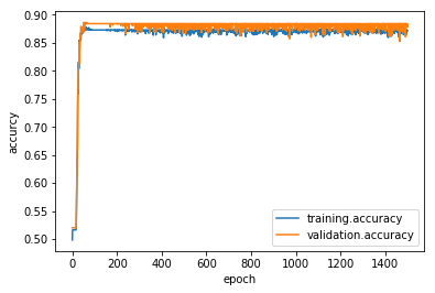
weights. Below we plot training and validation accuracies to confirm
that the weight regularization does not come at a cost of a signitficant
loss of accuracy.
In [9]:
fig, ax = plt.subplots(2,2, figsize=(12, 7))
ax = ax.flat

for i, experiment in enumerate(experiments):
    df = pd.DataFrame(data=np.array([experiment.metrics['training.accuracy'].values, experiment.metrics['validation.accuracy'].values]).T,
                  index=experiment.metrics['validation.accuracy'].index,
                  columns=['train_acc', 'val_acc'])

    df.plot(linestyle='', marker='.', markersize=5, ax=ax[i])
    ax[i].set_title(format_config(experiment.config, *differing_config_keys),
                    fontsize=12)
    ax[i].set_ylim([0,1])
    ax[i].set(xlabel='epoch', ylabel='accuracy')

plt.tight_layout()
plt.show()
Mutual information with the input for deterministic networks is currently calculated as the entropy of the representation. The representation in this context is the (histogram of the) activation pattern resulting from display of all input samples to the network in a specific epoch. A process towards a lower entropy activity distribution is therefore termed “compression”.
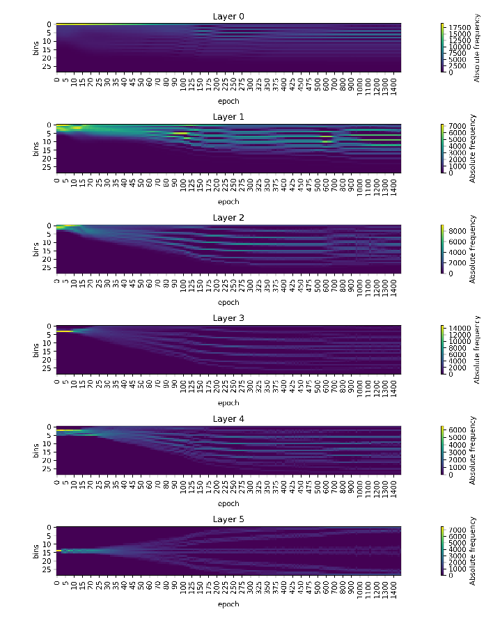
We now look at the average activations over epochs for each layer. Each column for the plots is a non-normalized histogram with 30 bins of the activations that were recorded during training and testing of the network.
In [6]:
fig, ax = plt.subplots(2,2, figsize=(25, 35))
ax = ax.flat

for i, experiment in enumerate(experiments):
    img = plt.imread(BytesIO(experiment.artifacts['activations'].content))
    ax[i].axis('off')
    ax[i].imshow(img)
    ax[i].set_title(format_config(experiment.config, *differing_config_keys),
                    fontsize=20)

plt.tight_layout()
plt.show()
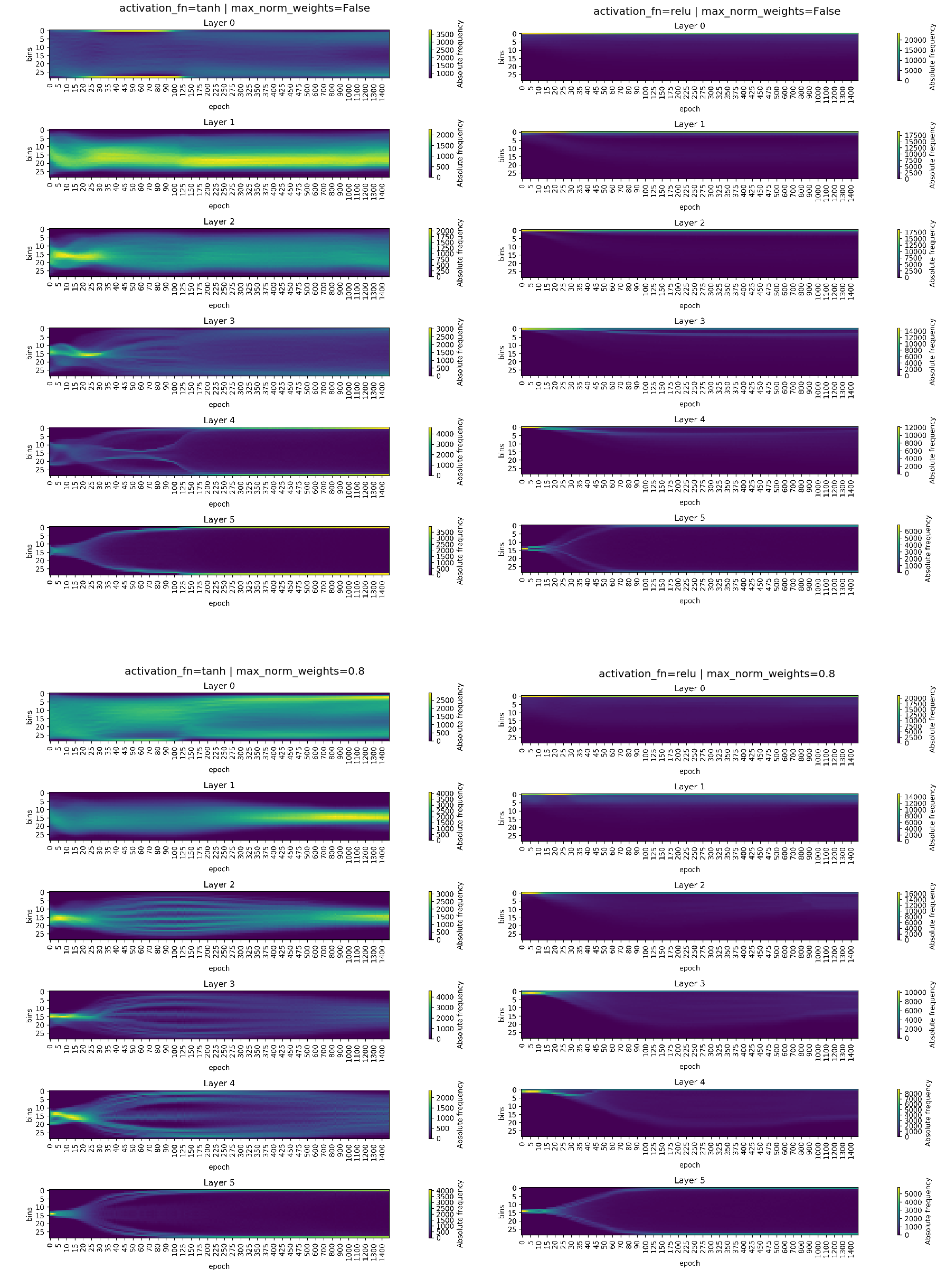
In the activation plots for tanh we can identify several very
prominent peaks of activations, especially during epochs 30-120 for
normal tanh and 30-250 for weight-restricted tanh. These
activity patterns conincide with the early phase of compression in the
tanh informationplane plots. Towards the end of training, higher
layers saturate and have peaks at activations of -1 and 1 in the
histograms. This phase also displays as compression in the
informationplane plot.
With regards to relu, the unconstrained network exhibits a peak of
activations at 0. In tendency, the remaining nonzero activations grow
over the course of training and spread a broader range. This
distribution has little structure (except for the prominent peak at 0)
and congruent with this also does not show compression in the
informationplane. The bias towards the entropy of the prominent peak at
0 due to the relu activation function will be discussed in more
detail in another notebook.
In the experiment with relu and with constrained weight vector, the
nonzero activations in the higher layers, especially in layer 3 and 4,
show several relatively pronounced peaks. They do not seem to be very
prominent, because there is still an big portion of all activations at
0. The pattern of several equidistant peaks of activation is similar to
the one observed in weight constrained tanh plots. Again, this is a
process towards a lower entropy distribution, which is reflected by the
observed “compression” in the information plane.
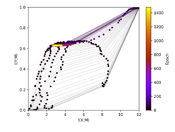
Experiment with max_weight_norm=0.4
In the following we present an example with relu and the norm of the
weight vector for each layer restricted to 0.4 This is a significantly
stronger regularization which this time will also have an effect on the
performance of the network.
In [12]:
relu04 = loader.find_by_id(603)
relu04.config
Out[12]:
{'activation_fn': 'relu',
 'architecture': [10, 7, 5, 4, 3],
 'batch_size': 256,
 'calculate_mi_for': 'full_dataset',
 'callbacks': [],
 'dataset': 'datasets.harmonics',
 'discretization_range': 0.07,
 'epochs': 1500,
 'estimator': 'mi_estimator.binning',
 'learning_rate': 0.0004,
 'max_norm_weights': 0.4,
 'model': 'models.feedforward',
 'n_runs': 1,
 'optimizer': 'adam',
 'plotters': [['plotter.informationplane', []],
  ['plotter.snr', []],
  ['plotter.informationplane_movie', []],
  ['plotter.activations', []],
  ['plotter.activations_single_neuron', []]],
 'seed': 42}
In the infoplane plot below it can be seen that training is impaired for the choice of such strict weight regularization.
In [8]:
relu04.artifacts['infoplane'].show()
Out[8]:
In [9]:
relu04.artifacts['activations'].show(figsize=(12,16))
Out[9]:
The activation pattern of several peaks is even more pronounced with stronger restiction on the size of the weights.
The performance of the network is worse than with higher weightnorm. But the training dynamics still look ok. The network learns the task up to a certain accurcy without overfitting.
In [15]:
relu04.metrics['training.accuracy'].plot()
relu04.metrics['validation.accuracy'].plot()
plt.ylabel('accurcy')
plt.xlabel('epoch')
plt.legend()
Out[15]:
<matplotlib.legend.Legend at 0x7f9c33efb978>
Supplementary material
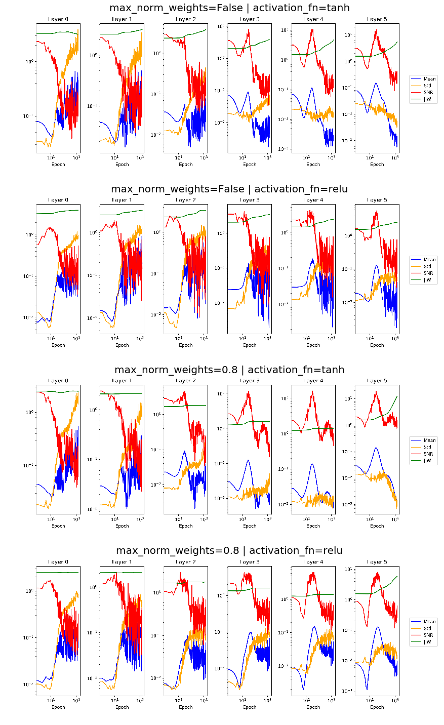
Below we find plots indicating the development of means and standard deviation of the gradient, its signal to noise ratio as well as the norm of the weight vector for all layers over the course of training. Comparing plots for unconstrained vs. constrained weight vector, we can reassure ourselves that rescaling the weights worked as we expected.
In [10]:
fig, ax = plt.subplots(4,1, figsize=(16, 20))
ax = ax.flat

for i, experiment in enumerate(experiments):
    img = plt.imread(BytesIO(experiment.artifacts['snr'].content))
    ax[i].axis('off')
    ax[i].imshow(img)
    ax[i].set_title(format_config(experiment.config, *differing_config_keys),
                    fontsize=20)

plt.tight_layout()
plt.show()
Below we find the configuration of all non-varied parameters that we used for the experiments above.
In [10]:
variable_config_dict = {k: '<var>' for k in differing_config_keys}
config = experiment.config
config.update(variable_config_dict)
config
Out[10]:
{'activation_fn': '<var>',
 'architecture': [10, 7, 5, 4, 3],
 'batch_size': 256,
 'calculate_mi_for': 'full_dataset',
 'callbacks': [],
 'dataset': 'datasets.harmonics',
 'discretization_range': 0.07,
 'epochs': 1500,
 'estimator': 'mi_estimator.binning',
 'learning_rate': 0.0004,
 'max_norm_weights': '<var>',
 'model': 'models.feedforward',
 'n_runs': 1,
 'optimizer': 'adam',
 'plotters': [['plotter.informationplane', []],
  ['plotter.snr', []],
  ['plotter.informationplane_movie', []],
  ['plotter.activations', []],
  ['plotter.activations_single_neuron', []]],
 'seed': 42}