The data set provided by Tishby

First, we load the data set provided by Tishby.

import os
import sys
nb_dir = os.path.split(os.path.split(os.getcwd())[0])[0]
sys.path.append(nb_dir)
from iclr_wrap_up.datasets import harmonics
import numpy as np

train_data, test_data = harmonics.load(nb_dir = nb_dir + '/iclr_wrap_up/')
X = np.concatenate([train_data[0], test_data[0]])
Y = np.concatenate([train_data[2], test_data[2]])

Next, we analyze the loaded data set. In this data set, \(X\) corresponds to the 12 binary inputs that represent 12 uniformly distributed points on a 2-sphere. \(X\) is realized as one of the 4096 possible combinations of the 12 binary inputs. \(Y\) corresponds to \(\Theta\left(f\left(X\right) - \theta\right)\), where \(f\) is a spherically symmetric real-valued function, \(\theta\) is a threshold, \(\Theta\) a step function that outputs either \(0\) or \(1\).

We sum over the 12 binary inputs of \(X\) and determine the share of \(Y=1\) per each possible sum value.

X_sum_Y = []

for i in range(13):
    X_sum_Y.append([])

for i in range(len(X)):
    n_pos_inputs = np.sum(X[i])
    X_sum_Y[n_pos_inputs].append(Y[i])

print('Share of Y=1 per each value of the sum of the binary inputs of X:')
for i in range(13):
    proportion = 100 * np.sum(np.array(X_sum_Y[i]))/len(X_sum_Y[i])
    print(f'{i}: {proportion}%')

Share of Y=1 per each value of the sum of the binary inputs of X:
0: 0.0%
1: 0.0%
2: 0.0%
3: 0.0%
4: 0.0%
5: 7.575757575757576%
6: 57.57575757575758%
7: 92.42424242424242%
8: 100.0%
9: 100.0%
10: 100.0%
11: 100.0%
12: 100.0%

Our attempt to generate the data set above

After analyzing the provided data set, we try to generate a similar one ourselves since the explicit algorithm for doing so was not provided in the paper.

The first task is to sample 12 uniformly distributed points on a unit 2-sphere. For that purpose, we randomly sample \(\theta\) from \([0, 2\pi]\) using the uniform distribution. Then, we randomly sample a value for the cosine of \(\phi\) from \([-1, 1]\) again using the uniform distribution. Finally, we apply arccosine to the sampled cosine of \(\phi\) to get \(\phi\) itself. Contrary to the convention, we have assigned \(\theta\) to the aziumthal angle and \(\phi\) to the polar angle to keep the naming consistent with SciPy’s spherical harmonics implementation.

Alternatively, one can randomly sample a 3-dimensional vector from \(\mathbb{R}^3\) using standard normal distribution, normalize it, and convert Cartesian coordinates to spherical coordinates.

import random
from scipy.special import sph_harm

def sample_spherical(npoints):
    """Sample npoints uniformly distributed
    points on a unit 2-sphere
    """
    thetas = np.zeros(npoints)
    phis = np.zeros(npoints)
    for i in range(npoints):
        thetas[i] = random.uniform(0, 2*np.pi)
        cos_phi = random.uniform(-1, 1)
        phis[i] = np.arccos(cos_phi)
    return thetas, phis

def alternative_sample_spherical(npoints):
    """Sample npoints uniformly distributed
    points on a unit 2-sphere
    """
    vec = np.random.randn(3, npoints)
    vec /= np.linalg.norm(vec, axis=0)
    thetas = np.arctan2(vec[1], vec[0]) + np. pi
    phis = np.arccos(vec[2])
    return thetas, phis

def wrong_sample_spherical(npoints):
    """Sample npoints points on a unit 2-sphere
    """
    thetas = np.zeros(npoints)
    phis = np.zeros(npoints)
    for i in range(npoints):
        thetas[i] = random.uniform(0, 2*np.pi)
        phis[i] = random.uniform(0, np.pi)
    return thetas, phis

np.random.seed(2)
random.seed(0)
thetas, phis = sample_spherical(12)

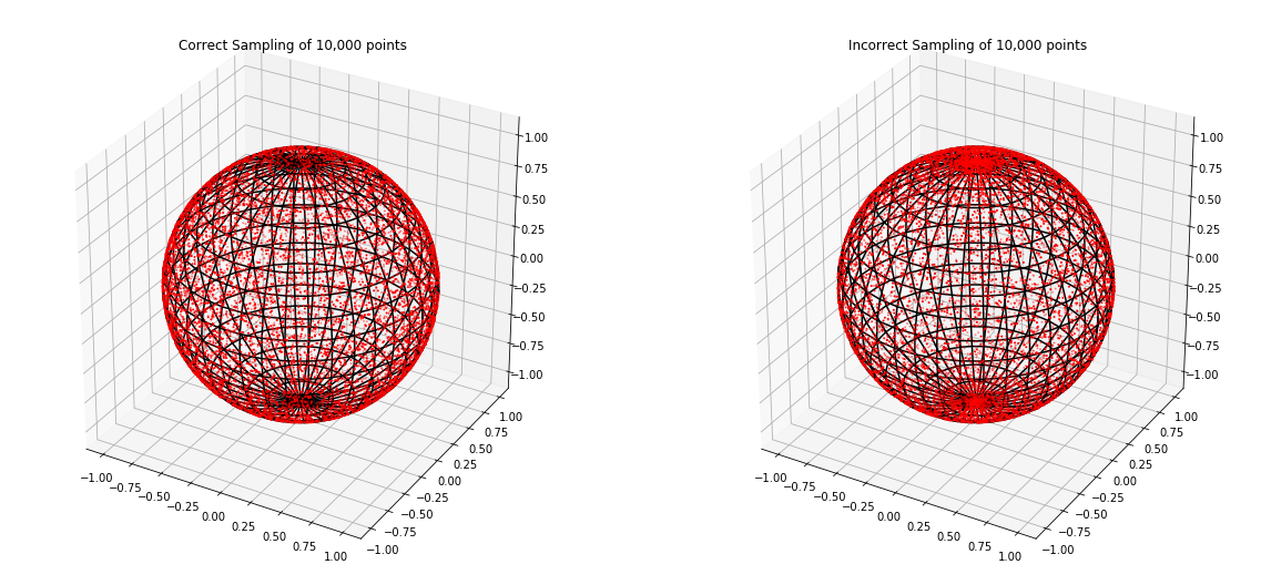
Directly sampling \(\phi\) from \([0, \pi]\) using uniform distribution results in concentration of points on the polar caps of the unit sphere (neighborhoods of \(z=1\) and \(z=-1\)). Note that to express the spherical coordinates \(\left(1, \phi, \theta\right)\) of a point on a unit sphere in terms of Cartesian coordinates \(\left(x, y, z\right)\), we use the formulas \(x = sin\left(\phi\right) \cdot cos\left(\theta\right)\), \(y = sin\left(\phi\right) \cdot sin\left(\theta\right)\), \(z = cos\left(\phi\right)\). Because \(cos\left(\phi\right)\) is flat near \(\phi = 0\) (\(z = cos\left(\phi\right) \approx 1\)) and \(\phi = \pi\) (\(z = cos\left(\phi\right) \approx -1\)) and \(sin\left(\phi\right)\) is almost zero near \(\phi = 0\) and \(\phi = \pi\) (\(x = sin\left(\phi\right) \cdot cos\left(\theta\right) \approx 0\) and \(y = sin\left(\phi\right) \cdot sin\left(\theta\right) \approx 0\)), higher than the expected share (under uniform distribution) of the sampled points will be concentrated on the northern (\(\left(x, y, z\right) \approx \left(0, 0, 1\right)\)) and southern (\(\left(x, y, z\right) \approx \left(0, 0, -1\right)\) polar caps of the unit sphere.

%matplotlib inline
from matplotlib import pyplot as plt
from mpl_toolkits.mplot3d import axes3d

correct_thetas, correct_phis = sample_spherical(10000)
wrong_thetas, wrong_phis = wrong_sample_spherical(10000)

phi = np.linspace(0, np.pi, 20)
theta = np.linspace(0, 2 * np.pi, 40)
x = np.outer(np.sin(theta), np.cos(phi))
y = np.outer(np.sin(theta), np.sin(phi))
z = np.outer(np.cos(theta), np.ones_like(phi))

correct_x = np.sin(correct_phis) * np.cos(correct_thetas)
correct_y = np.sin(correct_phis) * np.sin(correct_thetas)
correct_z = np.cos(correct_phis) * np.ones_like(correct_thetas)

wrong_x = np.sin(wrong_phis) * np.cos(wrong_thetas)
wrong_y = np.sin(wrong_phis) * np.sin(wrong_thetas)
wrong_z = np.cos(wrong_phis) * np.ones_like(wrong_thetas)

fig, ax = plt.subplots(1, 2, subplot_kw={'projection':'3d', 'aspect':'equal'}, figsize=(20,20))
ax[0].plot_wireframe(x, y, z, color='k', rstride=1, cstride=1)
ax[0].scatter(correct_x, correct_y, correct_z, s=1, c='r', zorder=1)
ax[0].set_title('Correct Sampling of 10,000 points')
ax[1].plot_wireframe(x, y, z, color='k', rstride=1, cstride=1)
ax[1].scatter(wrong_x, wrong_y, wrong_z, s=1, c='r', zorder=1)
ax[1].set_title('Incorrect Sampling of 10,000 points')
plt.show()

Next, we have to generate expansion coefficients \(a_{nm}\) for the spherical harmonic decomposition of the spherical function that underlies our spherically symmetric real-valued function \(f\).

def generate_coeffs(l):
    """Generate random expansion coefficients
    for the spherical harmonic decomposition
    up to l-th degree
    """
    coeffs = []
    # 0-th coefficient is 1.
    coeffs.append([1])
    for n in range(1, l+1):
        coeff = []
        for m in np.linspace(-n, n, 2*n + 1, dtype=int):
            # The rest of the coefficients are randomly
            # sampled from a standard normal distribution.
            coeff.append(np.random.randn())
        coeffs.append(coeff)
    return coeffs

# We generate coefficients up to 85th degree,
# since starting from 86, certain orders of the
# degree result in undefined coefficient values.
a_nm = generate_coeffs(85)

Now, we simulate the spherically symmetric real-valued function \(f\) using the generated coefficients \(a_{nm}\), the upper limit on the degree of the spherical harmonic decomposition \(l\), and inputs \(\theta\) and \(\phi\). For that purpose, we use Kazhdan’s rotation invariant descriptors, i.e., the energies of a spherical function \(g\), \(SH\left(g\right) = \left\{\left\|g_{0}\left(\theta, \phi\right)\right\|, \left\|g_{1}\left(\theta, \phi\right)\right\|, ...\right\}\) where \(g_n\) are the frequency components of \(g\):

\[ \begin{align}\begin{aligned}g_{n}\left(\theta, \phi\right) = \pi_{n}\left(g\right) = \sum_{m \ = \ n}^{-n} a_{nm} Y_{n}^{m}\left(\theta, \phi\right).\\In the equation above, :math:`\pi_n` is the projection onto the\end{aligned}\end{align} \]

subspace \(V_{n} = Span\left(Y_{n}^{-n},Y_{n}^{-n+1},...,Y_{n}^{n-1},Y_{n}^{n}\right)\), and \(Y_{n}^{m}\) is the spherical harmonic of degree \(n \geq 0\) and order \(\left|m\right| \leq n\). To process the pattern \(X\), we define \(f_l\) to be:

\[ \begin{align}\begin{aligned}f_l\left(X = \left(x_1, x_2, ..., x_{12}\right)\right) = \sum_{n \ = \ 0}^{l}\left\|\sum_{i \ = \ 1}^{12}x_i \cdot g_{n}\left(\theta_i, \phi_i\right)\right\|\\where :math:`\forall \ i: \ x_i \in \left\{0, 1\right\}`.\end{aligned}\end{align} \]

def func(a_nm, l, thetas, phis):
    """Apply f_l as defined above to the
    inputs thetas and phis using the
    decomposition coefficients a_nm
    """
    result = 0
    # the first summation
    for n in range(l+1):
        result_n = 0
        # the second summation
        for (theta, phi) in zip(thetas, phis):
            # the third summation corresponding to the freqency
            # component of the function
            for m in np.linspace(-n, n, 2*n + 1, dtype=int):
                result_n += a_nm[n][m] * sph_harm(m, n, theta, phi)
        # L2 norm
        result += np.linalg.norm(result_n)
    return result

Now, we assume \(f = f_{85}\) which implies that the expansion coefficients of the 86th degree and on are all zero. To find the appropriate \(\theta\) value for \(\Theta\left(f\left(X\right) - \theta\right)\), we look at our analysis of the provided data above. We see that the sum values between 0 and 4 involving the 12 binary inputs of \(X\) correspond to \(Y = 0\), and the sum values between 8 and 12 to \(Y = 1\). We also see that roughly 57.58% of the data points corresponding to the sum value of 6 result in \(Y = 1\). Hence, we assign the 42.42nd percentile (roughly 468.67) of \(f_{85}(X_6)\) (\(X_6\) corresponds to the data points with sum value of 6) to \(\theta\). We get binary \(\hat{Y}\) values through \(\hat{Y} = \Theta\left(f_{85}\left(X\right) - 468.67\right)\). In the end, we calculate the share of \(\hat{Y}=1\) per each value of the sum of the binary inputs of \(X\). As you can see below, the resulting numbers roughly mirror the ones we got above using the provided data set.

X_sum_Y_hat = []

for i in range(13):
    X_sum_Y_hat.append([])

for i in range(len(X)):
    n_pos_inputs = np.sum(X[i])
    X_sum_Y_hat[n_pos_inputs].append(func(a_nm, 85, thetas[X[i].astype(bool)], phis[X[i].astype(bool)]))

threshold = np.percentile(X_sum_Y_hat[6], 42.42)
print('\u03B8 \u2248 ' + str(np.around(threshold, decimals = 2)))

print('')

print('Share of \u0398(f(X)-\u03B8)=1 per each value of the sum of the binary inputs of X:')
for i in range(13):
    proportion = 100 * np.sum(np.array(X_sum_Y_hat[i]) > threshold)/len(X_sum_Y_hat[i])
    print(f'{i}: {proportion}%')

θ ≈ 468.67

Share of Θ(f(X)-θ)=1 per each value of the sum of the binary inputs of X:
0: 0.0%
1: 0.0%
2: 0.0%
3: 0.0%
4: 0.0%
5: 9.848484848484848%
6: 57.57575757575758%
7: 96.08585858585859%
8: 100.0%
9: 100.0%
10: 100.0%
11: 100.0%
12: 100.0%

In the next step, we soften \(\hat{Y} = \Theta\left(f\left(X\right) - \theta\right)\) to \(p\left(\hat{Y}=1\ \ | \ X \right) = \psi\left(f\left(X\right) - \theta\right)\) where \(\psi\left(u\right) = \frac{1}{1+e^{-\gamma \cdot u}}\). Here, \(\gamma\) is the sigmoidal gain and it should be high enough to keep the mutual information \(I\left(X \ ; \ \hat{Y}\right) \approx 0.99\) bits. We set \(\gamma\) to 1. We also assume that the selected \(\theta \approx 468.67\) results in \(p\left(\hat{Y}=1\right)=\sum_{X}p\left(\hat{Y}=1 \ | \ X \right) \cdot p\left(X\right) \approx 0.5\) with uniform \(p\left(X\right)\). As you can see below, the values we get for \(I\left(X \ ; \ \hat{Y}\right)\) and \(p\left(\hat{Y}=1\right)\) do meet the requirements.

def sigmoidal_func(u, gamma=1):
    """Sigmoidal function with
    the sigmoidal gain gamma
    """
    return 1/(1 + np.exp(-gamma*u))

# Here we calculate p(Y^hat = 1)
p_Y_hat = 0
p_X = 1/4096
for i in range(13):
    p_Y_hat += np.sum(sigmoidal_func(np.array(X_sum_Y_hat[i]) - threshold))
p_Y_hat *= p_X
print('p(\u0176=1) \u2248 ' + str(np.around(p_Y_hat, decimals = 1)))

# Here we calculate H(Y^hat)
H_Y_hat = -p_Y_hat*np.log2(p_Y_hat)-(1-p_Y_hat)*np.log2(1-p_Y_hat)
print('H(\u0176) \u2248 ' + str(np.around(H_Y_hat, decimals = 2)))

# Here we calculate H(Y^hat|X)
H_Y_hat_given_X = 0
p_X = 1/4096
for i in range(13):
    p_Y_hat_given_X = sigmoidal_func(np.array(X_sum_Y_hat[i]) - threshold)
    H_Y_hat_given_X -= np.sum(p_Y_hat_given_X*np.log2(p_Y_hat_given_X))
H_Y_hat_given_X *= p_X
print('H(\u0176|X) \u2248 ' + str(np.around(H_Y_hat_given_X, decimals = 2)))

# Here we calculate I(X;Y^hat) = H(Y^hat) - H(Y^hat|X)
I_X_Y_hat = H_Y_hat - H_Y_hat_given_X
print('I(X;\u0176) = H(\u0176) - H(\u0176|X) \u2248 '
      + str(np.around(H_Y_hat, decimals = 2)) + ' - '
      + str(np.around(H_Y_hat_given_X, decimals = 2)) + ' = '
      + str(np.around(I_X_Y_hat, decimals = 2)))

p(Ŷ=1) ≈ 0.5
H(Ŷ) ≈ 1.0
H(Ŷ|X) ≈ 0.01
I(X;Ŷ) = H(Ŷ) - H(Ŷ|X) ≈ 1.0 - 0.01 = 0.99